
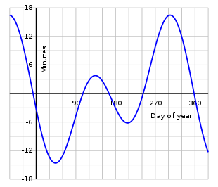
График уравнения времени (синяя линия) и двух его составляющих при определении этого уравнения как УВ = ССВ — ИСВ.

Уравнение времени (по «инвертированному» определению, принятому в англоязычной литературе). График выше нуля — солнечные часы «спешат», ниже нуля — солнечные часы «отстают»
Уравнение времени — разница между средним солнечным временем (ССВ) и истинным солнечным временем (ИСВ), то есть УВ = ССВ — ИСВ[1]. Эта разница в каждый конкретный момент времени одинакова для наблюдателя в любой точке Земли. Уравнение времени можно узнать из специализированных астрономических изданий, астрономических программ или вычислить по формуле, приведенной ниже.
В таких изданиях, как «Астрономический календарь», уравнение времени определяется как разность часовых углов среднего экваториального солнца и истинного солнца, то есть, при таком определении УВ = ССВ — ИСВ[2].
В англоязычных изданиях часто применяется иное определение уравнения времени (т. н. «инвертированное»): УВ = ИСВ — ССВ, то есть разница между истинным солнечным временем (ИСВ) и средним солнечным временем (ССВ).
Содержание
- 1 Некоторые пояснения к определению
- 2 Объяснение неравномерности движения истинного Солнца
- 2.1 Неравномерность, обусловленная эллиптичностью орбиты
- 2.2 Неравномерность, обусловленная наклоном земной оси
- 2.3 Уравнение времени как сумма обеих неравномерностей
- 3 Расчёт
- 3.1 Программа расчета на Ruby для текущей даты
- 4 См. также
- 5 Примечания
- 6 Ссылки
Некоторые пояснения к определению
Можно встретить определение уравнения времени как разницы «местного истинного солнечного времени» и «местного среднего солнечного времени» (в англоязычной литературе — local apparent solar time и local mean solar time). Данное определение формально более точно, но не влияет на результат, так как для любой конкретной точки на Земле эта разница одинакова.
Кроме того, не следует путать ни «местное истинное солнечное время», ни «местное среднее солнечное время» с официальным местным временем (standard time).
Объяснение неравномерности движения истинного Солнца
В отличие от звезд, чьё видимое суточное движение практически равномерно и обусловлено только вращением Земли вокруг своей оси, суточное движение Солнца не равномерно, так как обусловлено и вращением Земли вокруг своей оси, и вращением Земли вокруг Солнца, и наклоном земной оси к плоскости эклиптики.
Неравномерность, обусловленная эллиптичностью орбиты
Вращение Земли вокруг Солнца происходит по эллиптической орбите. Согласно второму закону Кеплера, такое движение неравномерно, оно быстрее в области перигелия и медленнее в области афелия. Для наблюдателя, находящегося на Земле, это выражается в том, что видимое движение Солнца по эклиптике относительно неподвижных звезд то ускоряется, то замедляется.
Неравномерность, обусловленная наклоном земной оси
Поскольку плоскость эклиптики наклонена к плоскости небесного экватора, имеет место следующее явление:
- Солнце вблизи солнцестояний (зимнего и летнего) движется почти параллельно к небесному экватору, и скорость его перемещения практически полностью вычитается из суточного движения небесной сферы — результирующая скорость изменения часового угла Солнца минимальна;
- Солнце вблизи равноденствий (осеннего и весеннего) движется под максимальным углом к небесному экватору, и скорость его перемещения лишь частично вычитается из суточного движения небесной сферы — результирующая скорость изменения часового угла Солнца максимальна.
Уравнение времени как сумма обеих неравномерностей

1. Влияние эксцентриситета 2. Влияние наклона эклиптики 3. Сумма — Уравнение времени 4. Позиция истинного Солнца относительно среднего Солнца.
(Графики приведены в соответствии с «инвертированным» определением уравнения времени, принятым в англоязычной литературе)
Кривая уравнения времени является суммой двух периодических кривых — с периодами 1 год и 6 месяцев. Практически синусоидальная кривая с годичным периодом обусловлена неравномерным движением Солнца по эклиптике. Эта часть уравнения времени называется уравнением центра или уравнением от эксцентриситета. Синусоида с периодом 6 месяцев представляет разность времён, вызванную наклоном эклиптики к небесному экватору и называется уравнением от наклона эклиптики[1].
Уравнение времени обращается в ноль четыре раза в году: 14 апреля, 14 июня, 2 сентября и 24 декабря.
Соответственно, в каждое время года существует свой максимум уравнения времени: около 12 февраля — +14,3 мин, 15 мая — −3,8 мин, 27 июля — +6,4 мин и 4 ноября — −16,4 мин. Точные величины уравнения времени даются в астрономических ежегодниках.
Может применяться как дополнительная функция в некоторых моделях часов.
Расчёт
Уравнение можно аппроксимировать отрезком ряда Фурье как сумму двух синусоидальных кривых с периодами, соответственно, на один год и шесть месяцев:

где
 если углы выражаются в градусах.

или
- если углы выражаются в радианах.

- Там, где — количество дней, например:

- на 1 января

- на 2 января

и так далее.
Программа расчета на Ruby для текущей даты
#!/usr/bin/ruby

=begin
Equation of Time calculation
    *** No guarantees are implied. Use at your own risk ***

    Written by E. Sevastyanov, 2017-05-14

    Based on "Equation of time" WikiPedia article as of 2016-11-28
    (which describes angles in a bewildering mixture of degrees and radians)
    and
    Del Smith, 2016-11-29

    It appears to give a good result, but I make no claims for accuracy.
=end

pi = (Math::PI) # pi
delta = (Time.now.getutc.yday - 1) # (Текущий день года - 1)

yy = Time.now.getutc.year
np = case yy #The number np is the number of days from 1 January to the date of the Earth's perihelion. (http://www.astropixels.com/ephemeris/perap2001.html)
when 2017 ; 3
when 2018 ; 2
when 2019 ; 2
when 2020 ; 4
when 2021 ; 1
when 2022 ; 3
when 2023 ; 3
when 2024 ; 2
when 2025 ; 3
when 2026 ; 2
when 2027 ; 2
when 2028 ; 4
when 2029 ; 1
when 2030 ; 2
else; 2
end

a = Time.now.getutc.to_a; delta = delta + a[2].to_f / 24 + a[1].to_f / 60 / 24 # Поправка на дробную часть дня

lambda = 23.4406 * pi / 180; # Earth's inclination in radians
omega = 2 * pi / 365.2564 # angular velocity of annual revolution (radians/day)
alpha = omega * ((delta + 10) % 365) # angle in (mean) circular orbit, solar year starts 21. Dec
beta = alpha + 0.03340560188317 * Math.sin(omega * ((delta - np) % 365)) # angle in elliptical orbit, from perigee  (radians)
gamma = (alpha - Math.atan(Math.tan(beta) / Math.cos(lambda))) / pi # angular correction
eot = (43200 * (gamma - gamma.round)) # equation of time in seconds
puts "EOT =" + (-1 * eot).to_s + " секунд"
См. также
- Аналемма
Примечания
- ↑ 1 2 Кононович Э. В., Мороз В. И. «Общий курс астрономии» Учебное пособие под ред. В. В. Иванова. Изд. 2-е, испр. М.: Едиториал УРСС, 2004. — 544 с. ISBN 5-354-00866-2, 3000 экз.
- ↑ Астрономический календарь. Постоянная часть / Ответственный редактор Абалакин В.К.. — 7-е изд. — М.: Наука, 1981. — С. 19.
Ссылки
- Величина колебаний уравнения времени в течение года на портале Гринвичской королевской обсерватории.
- Уравнение времени на сегодняшний день — визуализация.
- Образец построения графика уравнения времени, где прорисованы:
- 1 — составляющая уравнения времени, определяемая неравномерностью движения Земли по орбите,
- 2 — составляющая уравнения времени, определяемая наклоном эклиптики к экватору,
- 3 — уравнение времени.
Уравнение времени и аналемма
Солнечные часы принципиально отличаются от всех остальных инструментов
измерения времени. Дело в том, что они измеряют не одинаковые промежутки времени, как это делают все остальные часы, а
движение Солнца, что не одно и то же. Разница между средним временем и
солнечным описывается уравнением времени и составлет около ±15 минут.

Отображение разницы между солнечным временем и средним является крайне сложной задачей (и предметом гордости) для любого часовщика.
На фото слева изображены механические часы Notos Мартина Брауна, которые помимо даты отображают значение уравнения времени и
долготу Солнца.
Среднее время и фантомное Солнце

Все часы кроме солнечных
отмеряют одинаковые промежутки времени
и показывают среднее время.
Промежутками могут быть часы, минуты, секунды или миллисекунды.
Чем меньше разница между двумя одинаковыми отмеренными промежутками, тем часы точнее и, стало быть, лучше.
Если бы Солнце уподобилось точным часам,
то оно должно было бы вращаться вокруг Земли с постоянной скоростью по круговой орбите,
расположенной в плоскости экватора.
В последующих рассуждениях такое Солнце будет называться фантомным и обозначаться
на чертежах серым цветом и буквой f.
Все наши современные представления о времени и сама система его подсчета
основаны на движении этого самого фантомного Солнца,
которое обращается вокруг Земли с постоянной скоростью 24 часа в сутки.
И происходит это каждый день в течение всего года.
Однако в реальности орбита, по которой Солнце вращается вокруг Земли, эллиптическая,
а не круговая.
К тому же ось вращения Земли наклонена к плоскости вращения Солнца (эклиптике) под углом около 23,5°.
Именно эти два фактора приводят к тому, что реальное Солнце t ведет себя по-другому
и, наряду с фантомным средним временем, существует истинное время,
которое умеют показывать только солнечные часы.
На рисунке, приведенном выше, обозначены два положения Солнца, соответствующие одному моменту времени.
Фантомное Солнце f всегда движется по экватору с постоянной скоростью. Среднее местное время, которое
соответствует его положению, определяется углом hf,
который откладывается от направления на юг, то есть полудня.
В тоже время реальное Солнце t движется по эклиптике, которая пересекает экватор только
в дни равноденствия. На рисунке эклиптика и реальное Солнце обозначены оранжевым цветом, а
точка весеннего равноденствия буквой γ. Истинное время соответствует углу ht.
В общем случае эти углы не совпадают, и уравнение времени можно записать, как
ht — hf.
Описанное несоответствие среднего времени истинному имеет 6-месячный период и
равняется нулю четыре раза в год:
в дни равноденствия и солнцестояния.
За счет фактора несоответствия эклиптики экватору (то есть из-за наклона земной оси)
уравнение времени изменяется примерно от -9,87 до +9,87 минут в течение года.
Эллиптическая орбита и законы Кеплера
Вторая причина несоответствия среднего времени истинному,
то есть уравнения времени, заключается в том,
что годовое движение Солнца вокруг Земли происходит по эллиптической, а не круговой орбите.

В начале XVII века немецкий астроном Иоганн Кеплер открыл три закона вращения планет,
из которых к уравнению времени имеют отношение первые два. Первый закон
описывает все возможные орбиты движения небесных тел относительно друг друга.
В частности, при огибании Солнцем Земли по эллиптической орбите Земля располагается в одном из
фокусов данного эллипса, как изображено на рисунке слева. При этом точка 1 соответствует
максимальному удалению Солнца от Земли и называется апогей. Минимальное расстояние
между Землей и Солнцем достигается в точке 2, называемой перигей.
Ближе всего Солнце подходит к Земле 3 января, а дальше всего находится 4 июля.
Конечно, Солнце находится в одном из фокусов эллиптической орбиты, по которой Земля вращается вокруг него, но
с точки зрения гномоники этот факт лишь затрудняет понимание принципов работы солнечных часов.
Для тех, кто предпочитает рассматривать вращение Земли вокруг Солнца, следует заметить, что
ближайшая к Солнцу точка называется перигелий, а самая удаленная — афелий.
Второй закон Кеплера утверждает, что при движении Солнца по эллиптической орбите
его скорость не будет постоянной, а будет увеличиваться при приближении к Земле в точке
перигея и уменьшаться в точке апогея. Саму зависимость можно проиллюстрировать графически.
Солнце проходит участки AB и CD за одно и то же время в том случае, если
площади соответствующих затемненных участков равны.

На рисунке слева изображены положения двух Солнцев: фантомного f и истинного t.
Фантомное Солнце, определяющее среднее время, двигается вокруг Земли по круговой орбите с
постоянной скоростью. Реальное Солнце, напротив, ускоряется возле точки перигея 2 и
замедляется в апогее 1.
Соответственно, долгота фантомного и реального Солнца, которая выражается углом, отложенным
от точки весеннего равноденствия γ, будет разной. Доля данного несоответствия среднего времени
истинному в уравнении времени выражается формулой Lt — Lf. Дважды
в год, в апогее и перигее, эта разница становится равной нулю, а в остальное время она изменяется от
-7,66 до +7,66 минут.
На приведенных рисунках эллиптичность орбиты намеренно подчеркнута,
хотя на самом деле эксцентриситет
земной орбиты составляет всего лишь 0, 017. Это означает, что орбита почти совпадает с окружностью, у
которой эксцентриситет равен 0. Однако, это «почти»
вносит серьезные изменения в скорость движения Солнца по эклиптике.
В январе его скорость составляет 1°01′ за 24 часа против 0°57′ в июле.
График уравнения времени

Таким образом, уравнение времени в основном складывается
из двух несоответствий между временем
средним и истинным, то есть солнечным. Первое несоответствие связано с наклоном земной оси.
А второе несоответствие проистекает
из того, что Солнце движется не по круговой, а по эллиптической орбите.
Поскольку сами несоответствия сложно синхронизированы и имеют разные значения, то
результирующий график уравнения времени, изображенный
на рисунке в начале, несимметричен относительно нулевого значения.
Уравнение времени принимает положительное значение, когда Солнце
пересекает локальный меридиан раньше, чем это сделало бы фантомное Солнце,
двигающееся равномерно по среднему времени. Отрицательное значение
означает, что истинное время опаздывает по сравнению со средним.
Как видно на графике значение уравнения времени равно нулю четыре раза в год:
15 апреля, 13 июня, 1 сентября и 25 декабря. Иногда график уравнения времени
рисуют инвертированным и уравнение времени представляется, как среднее время минус истинное.
Вообще-то несоответствий между Солнцем фантомным и реальным значительно больше
(известный популиризатор астрономии Фламарион описал еще 13 сложных движений Земли),
но основной и заметный вклад в уравнение времени связан с орбитой Земли и наклоном оси ее вращения .
Аналемматическая кривая

Иногда уравнение времени изображают в виде
аналемматической «восьмерки». В интернете можно найти фотографии, подобные
размещенной. Если установить фотоаппарат на штатив и производить мультиэкспозиционную съемку
каждый день в одно и тоже гражданское время, то Солнце в течение года опишет фигуру,
которая похожа на восьмерку.
Именно такую фигуру называют аналеммой. В зависимости от места
и времени съемки кривая может иметь разную форму и наклон. Например, если бы съемка велась
в 12:00 в Гринвиче, то аналемма располагалась бы строго вертикально.

Иногда на солнечных часах изображают аналемматическую восьмерку, которая позволяет согласовать среднее и
истинное время. Для этого надо знать, что полдень по среднему времени наступает, когда тень от конца гномона
пересекает соответствующую часть аналеммы. Одновременно по этой тени можно определить время года, как
это предполагается на часах МГУ на фотографии.

Если делаются солнечные часы, которые показывают точное среднее время, то при их разметке
следует учитывать уравнение времени. Поэтому часовые линии на таких часах всегда будут в виде
аналемматических кривых. Другой способ отображения среднего времени солнечными часами запечатлен на фотографии.
Армилярная полусфера имеет необычный гномон в виде прорезанной аналемматической восьмерки.
На изогнутой шкале представлены два времени: гражданское среднее сверху и истинное солнечное снизу.
The equation of time — above the axis a sundial will appear fast relative to a clock showing local mean time, and below the axis a sundial will appear slow.
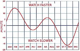
This graph shows how many minutes the clock is ahead (+) or behind (−) the apparent sun. See the section «Sign of the equation of time» below.
The equation of time describes the discrepancy between two kinds of solar time. The word equation is used in the medieval sense of «reconciliation of a difference». The two times that differ are the apparent solar time, which directly tracks the diurnal motion of the Sun, and mean solar time, which tracks a theoretical mean Sun with uniform motion along the celestial equator. Apparent solar time can be obtained by measurement of the current position (hour angle) of the Sun, as indicated (with limited accuracy) by a sundial. Mean solar time, for the same place, would be the time indicated by a steady clock set so that over the year its differences from apparent solar time would have a mean of zero.[1]
The equation of time is the east or west component of the analemma, a curve representing the angular offset of the Sun from its mean position on the celestial sphere as viewed from Earth. The equation of time values for each day of the year, compiled by astronomical observatories, were widely listed in almanacs and ephemerides.[2][3]: 14
The concept[edit]

Clock with auxiliary dial displaying the equation of time. Piazza Dante, Naples (1853).
During a year the equation of time varies as shown on the graph; its change from one year to the next is slight. Apparent time, and the sundial, can be ahead (fast) by as much as 16 min 33 s (around 3 November), or behind (slow) by as much as 14 min 6 s (around 11 February). The equation of time has zeros near 15 April, 13 June, 1 September, and 25 December. Ignoring very slow changes in the Earth’s orbit and rotation, these events are repeated at the same times every tropical year. However, due to the non-integral number of days in a year, these dates can vary by a day or so from year to year.[n 1][4]: 277
The graph of the equation of time is closely approximated by the sum of two sine curves, one with a period of a year and one with a period of half a year. The curves reflect two astronomical effects, each causing a different non-uniformity in the apparent daily motion of the Sun relative to the stars:
- the obliquity of the ecliptic (the plane of the Earth’s annual orbital motion around the Sun), which is inclined by about 23.44 degrees relative to the plane of the Earth’s equator; and
- the eccentricity of the Earth’s orbit around the Sun, which is about 0.0167.
The equation of time vanishes only for a planet with zero axial tilt and zero orbital eccentricity.[5] Two examples of planets with large equations of time are Mars and Uranus. On Mars the difference between sundial time and clock time can be as much as 50 minutes, due to the considerably greater eccentricity of its orbit. The planet Uranus, which has an extremely large axial tilt, has an equation of time that makes its days start and finish several hours earlier or later depending on where it is in its orbit.
Sign of the equation of time[edit]
The United States Naval Observatory states «the Equation of Time is the difference apparent solar time minus mean solar time«, i.e. if the sun is ahead of the clock the sign is positive, and if the clock is ahead of the sun the sign is negative.[6][7] The equation of time is shown in the upper graph above for a period of slightly more than a year. The lower graph (which covers exactly one calendar year) has the same absolute values but the sign is reversed as it shows how far the clock is ahead of the sun. Publications may use either format — in the English-speaking world, the former usage is the more common, but is not always followed. Anyone who makes use of a published table or graph should first check its sign usage. Often, there is a note or caption which explains it. Otherwise, the usage can be determined by knowing that, during the first three months of each year, the clock is ahead of the sundial. The mnemonic «NYSS» (pronounced «nice»), for «new year, sundial slow», can be useful. Some published tables avoid the ambiguity by not using signs, but by showing phrases such as «sundial fast» or «sundial slow» instead.[8]
In this article, and others in English Wikipedia, a positive value of the equation of time implies that a sundial is ahead of a clock.
History[edit]
The phrase «equation of time» is derived from the medieval Latin aequātiō diērum, meaning «equation of days» or «difference of days».
The word aequātiō (and Middle English equation) was used in medieval astronomy to tabulate the difference between an observed value and the expected value (as in the equation of the centre, the equation of the equinoxes, the equation of the epicycle).
Gerald J. Toomer uses the medieval term «equation», from the Latin aequātiō,[n 2] for Ptolemy’s difference between the mean solar time and the apparent solar time. Johannes Kepler’s definition of the equation is «the difference between the number of degrees and minutes of the mean anomaly and the degrees and minutes of the corrected anomaly.»[9]: 155
The difference between apparent solar time and mean time was recognized by astronomers since antiquity, but prior to the invention of accurate mechanical clocks in the mid-17th century, sundials were the only reliable timepieces, and apparent solar time was the generally accepted standard. Mean time did not supplant apparent time in national almanacs and ephemerides until the early 19th century. [10]
Early astronomy[edit]
The irregular daily movement of the Sun was known to the Babylonians.[citation needed]
Book III of Ptolemy’s Almagest (2nd century) is primarily concerned with the Sun’s anomaly, and he tabulated the equation of time in his Handy Tables.[11] Ptolemy discusses the correction needed to convert the meridian crossing of the Sun to mean solar time and takes into consideration the nonuniform motion of the Sun along the ecliptic and the meridian correction for the Sun’s ecliptic longitude. He states the maximum correction is 8+1⁄3 time-degrees or 5⁄9 of an hour (Book III, chapter 9).[12] However he did not consider the effect to be relevant for most calculations since it was negligible for the slow-moving luminaries and only applied it for the fastest-moving luminary, the Moon.
Based on Ptolemy’s discussion in the Almagest, values for the equation of time (Arabic taʿdīl al-ayyām bi layālayhā) were standard for the tables (zij) in the works of medieval Islamic astronomy.[13]
Early modern period[edit]
A description of apparent and mean time was given by Nevil Maskelyne in the Nautical Almanac for 1767: «Apparent Time is that deduced immediately from the Sun, whether from the Observation of his passing the Meridian, or from his observed Rising or Setting. This Time is different from that shewn by Clocks and Watches well regulated at Land, which is called equated or mean Time.» He went on to say that, at sea, the apparent time found from observation of the Sun must be corrected by the equation of time, if the observer requires the mean time.[1]
The right time was originally considered to be that which was shown by a sundial. When good mechanical clocks were introduced, they agreed with sundials only near four dates each year, so the equation of time was used to «correct» their readings to obtain sundial time. Some clocks, called equation clocks, included an internal mechanism to perform this «correction». Later, as clocks became the dominant good timepieces, uncorrected clock time, i.e., «mean time», became the accepted standard. The readings of sundials, when they were used, were then, and often still are, corrected with the equation of time, used in the reverse direction from previously, to obtain clock time. Many sundials, therefore, have tables or graphs of the equation of time engraved on them to allow the user to make this correction.[8]: 123
The equation of time was used historically to set clocks. Between the invention of accurate clocks in 1656 and the advent of commercial time distribution services around 1900, there were several common land-based ways to set clocks. A sundial was read and corrected with the table or graph of the equation of time. If a transit instrument was available, the sun’s transit across the meridian (the moment the sun appears to be due south or north of the observer) was noted; the clock was then set to noon and offset by the number of minutes given by the equation of time for that date. A third method did not use the equation of time; instead, it used stellar observations to give sidereal time, exploiting the relationship between sidereal time and mean solar time.[14]: 57–58
The first tables to give the equation of time in an essentially correct way were published in 1665 by Christiaan Huygens.[15] Huygens, following the tradition of Ptolemy and medieval astronomers in general, set his values for the equation of time so as to make all values positive throughout the year.[15][n 3]
Another set of tables was published in 1672–73 by John Flamsteed, who later became the first Astronomer Royal of the new Royal Greenwich Observatory. These appear to have been the first essentially correct tables that gave today’s meaning of Mean Time (previously, as noted above, the sign of the equation was always positive and it was set at zero when the apparent time of sunrise was earliest relative to the clock time of sunrise). Flamsteed adopted the convention of tabulating and naming the correction in the sense that it was to be applied to the apparent time to give mean time.[16]
The equation of time, correctly based on the two major components of the Sun’s irregularity of apparent motion,[n 4] was not generally adopted until after Flamsteed’s tables of 1672–73, published with the posthumous edition of the works of Jeremiah Horrocks.[17]: 49
Robert Hooke (1635–1703), who mathematically analyzed the universal joint, was the first to note that the geometry and mathematical description of the (non-secular) equation of time and the universal joint were identical, and proposed the use of a universal joint in the construction of a «mechanical sundial».[18]: 219
18th and early 19th centuries[edit]
The corrections in Flamsteed’s tables of 1672–1673 and 1680 gave mean time computed essentially correctly and without need for further offset. But the numerical values in tables of the equation of time have somewhat changed since then, owing to three factors:
- general improvements in accuracy that came from refinements in astronomical measurement techniques,
- slow intrinsic changes in the equation of time, occurring as a result of small long-term changes in the Earth’s obliquity and eccentricity (affecting, for instance, the distance and dates of perihelion), and
- the inclusion of small sources of additional variation in the apparent motion of the Sun, unknown in the 17th century but discovered from the 18th century onwards, including the effects of the Moon,[n 5] Venus and Jupiter.[19]

From 1767 to 1833, the British Nautical Almanac and Astronomical Ephemeris tabulated the equation of time in the sense ‘add or subtract (as directed) the number of minutes and seconds stated to or from the apparent time to obtain the mean time’. Times in the Almanac were in apparent solar time, because time aboard ship was most often determined by observing the Sun. This operation would be performed in the unusual case that the mean solar time of an observation was needed. In the issues since 1834, all times have been in mean solar time, because by then the time aboard ship was increasingly often determined by marine chronometers. The instructions were consequently to add or subtract (as directed) the number of minutes stated to or from the mean time to obtain the apparent time. So now addition corresponded to the equation being positive and subtraction corresponded to it being negative.
As the apparent daily movement of the Sun is one revolution per day, that is 360° every 24 hours, and the Sun itself appears as a disc of about 0.5° in the sky, simple sundials can be read to a maximum accuracy of about one minute. Since the equation of time has a range of about 33 minutes, the difference between sundial time and clock time cannot be ignored. In addition to the equation of time, one also has to apply corrections due to one’s distance from the local time zone meridian and summer time, if any.
The tiny increase of the mean solar day due to the slowing down of the Earth’s rotation, by about 2 ms per day per century, which currently accumulates up to about 1 second every year, is not taken into account in traditional definitions of the equation of time, as it is imperceptible at the accuracy level of sundials.
Major components of the equation[edit]
Eccentricity of the Earth’s orbit[edit]

Equation of time (red solid line) and its two main components plotted separately, the part due to the obliquity of the ecliptic (mauve dashed line) and the part due to the Sun’s varying apparent speed along the ecliptic due to eccentricity of the Earth’s orbit (dark blue dash & dot line)
The Earth revolves around the Sun. As seen from Earth, the Sun appears to revolve once around the Earth through the background stars in one year. If the Earth orbited the Sun with a constant speed, in a circular orbit in a plane perpendicular to the Earth’s axis, then the Sun would culminate every day at exactly the same time, and be a perfect time keeper (except for the very small effect of the slowing rotation of the Earth). But the orbit of the Earth is an ellipse not centered on the Sun, and its speed varies between 30.287 and 29.291 km/s, according to Kepler’s laws of planetary motion, and its angular speed also varies, and thus the Sun appears to move faster (relative to the background stars) at perihelion (currently around 3 January) and slower at aphelion a half year later.[20][21][22]
At these extreme points this effect varies the apparent solar day by 7.9 s/day from its mean. Consequently, the smaller daily differences on other days in speed are cumulative until these points, reflecting how the planet accelerates and decelerates compared to the mean. As a result, the eccentricity of the Earth’s orbit contributes a periodic variation which is (in the first-order approximation) a sine wave with an amplitude of 7.66 min and a period of one year to the equation of time. The zero points are reached at perihelion (at the beginning of January) and aphelion (beginning of July); the extreme values are in early April (negative) and early October (positive).
Obliquity of the ecliptic[edit]

Sun and planets at local apparent noon (Ecliptic in red, Sun and Mercury in yellow, Venus in white, Mars in red, Jupiter in yellow with red spot, Saturn in white with rings).
Even if the Earth’s orbit were circular, the perceived motion of the Sun along our celestial equator would still not be uniform.[5] This is a consequence of the tilt of the Earth’s rotational axis with respect to the plane of its orbit, or equivalently, the tilt of the ecliptic (the path the Sun appears to take in the celestial sphere) with respect to the celestial equator. The projection of this motion onto our celestial equator, along which «clock time» is measured, is a maximum at the solstices, when the yearly movement of the Sun is parallel to the equator (causing amplification of perceived speed) and yields mainly a change in right ascension. It is a minimum at the equinoxes, when the Sun’s apparent motion is more sloped and yields more change in declination, leaving less for the component in right ascension, which is the only component that affects the duration of the solar day. A practical illustration of obliquity is that the daily shift of the shadow cast by the Sun in a sundial even on the equator is smaller close to the solstices and greater close to the equinoxes. If this effect operated alone, then days would be up to 24 hours and 20.3 seconds long (measured solar noon to solar noon) near the solstices, and as much as 20.3 seconds shorter than 24 hours near the equinoxes.[20][23][22]
In the figure on the right, we can see the monthly variation of the apparent slope of the plane of the ecliptic at solar midday as seen from Earth. This variation is due to the apparent precession of the rotating Earth through the year, as seen from the Sun at solar midday.
In terms of the equation of time, the inclination of the ecliptic results in the contribution of a sine wave variation with an amplitude of 9.87 minutes and a period of a half year to the equation of time. The zero points of this sine wave are reached at the equinoxes and solstices, while the extrema are at the beginning of February and August (negative) and the beginning of May and November (positive).
Secular effects[edit]
The two above mentioned factors have different wavelengths, amplitudes and phases, so their combined contribution is an irregular wave. At epoch 2000 these are the values (in minutes and seconds with UT dates):
| Point | Value | Date |
|---|---|---|
| minimum | −14 min 15 s | 11 February |
| zero | 0 min 00 s | 15 April |
| maximum | +3 min 41 s | 14 May |
| zero | 0 min 00 s | 13 June |
| minimum | −6 min 30 s | 26 July |
| zero | 0 min 00 s | 1 September |
| maximum | +16 min 25 s | 3 November |
| zero | 0 min 00 s | 25 December |
[citation needed]
- E.T. = apparent − mean. Positive means: Sun runs fast and culminates earlier, or the sundial is ahead of mean time. A slight yearly variation occurs due to presence of leap years, resetting itself every 4 years. The exact shape of the equation of time curve and the associated analemma slowly change over the centuries, due to secular variations in both eccentricity and obliquity. At this moment both are slowly decreasing, but they increase and decrease over a timescale of hundreds of thousands of years.[24]
On shorter timescales (thousands of years) the shifts in the dates of equinox and perihelion will be more important. The former is caused by precession, and shifts the equinox backwards compared to the stars. But it can be ignored in the current discussion as our Gregorian calendar is constructed in such a way as to keep the vernal equinox date at 20 March (at least at sufficient accuracy for our aim here). The shift of the perihelion is forwards, about 1.7 days every century. In 1246 the perihelion occurred on 22 December, the day of the solstice, so the two contributing waves had common zero points and the equation of time curve was symmetrical: in Astronomical Algorithms Meeus gives February and November extrema of 15 m 39 s and May and July ones of 4 m 58 s. Before then the February minimum was larger than the November maximum, and the May maximum larger than the July minimum. In fact, in years before −1900 (1901 BCE) the May maximum was larger than the November maximum. In the year −2000 (2001 BCE) the May maximum was +12 minutes and a couple seconds while the November maximum was just less than 10 minutes. The secular change is evident when one compares a current graph of the equation of time (see below) with one from 2000 years ago, e.g., one constructed from the data of Ptolemy.[25]
Graphical representation[edit]
Animation showing equation of time and analemma path over one year.
Practical use[edit]
If the gnomon (the shadow-casting object) is not an edge but a point (e.g., a hole in a plate), the shadow (or spot of light) will trace out a curve during the course of a day. If the shadow is cast on a plane surface, this curve will be a conic section (usually a hyperbola), since the circle of the Sun’s motion together with the gnomon point define a cone. At the spring and fall equinoxes, the cone degenerates into a plane and the hyperbola into a line. With a different hyperbola for each day, hour marks can be put on each hyperbola which include any necessary corrections. Unfortunately, each hyperbola corresponds to two different days, one in each half of the year, and these two days will require different corrections. A convenient compromise is to draw the line for the «mean time» and add a curve showing the exact position of the shadow points at noon during the course of the year. This curve will take the form of a figure eight and is known as an analemma. By comparing the analemma to the mean noon line, the amount of correction to be applied generally on that day can be determined.
The equation of time is used not only in connection with sundials and similar devices, but also for many applications of solar energy. Machines such as solar trackers and heliostats have to move in ways that are influenced by the equation of time.
Civil time is the local mean time for a meridian that often passes near the center of the time zone, and may possibly be further altered by daylight saving time. When the apparent solar time that corresponds to a given civil time is to be found, the difference in longitude between the site of interest and the time zone meridian, daylight saving time, and the equation of time must all be considered.[26]
Calculating the equation of time[edit]
The equation of time is obtained from a published table, or a graph. For dates in the past such tables are produced from historical measurements, or by calculation; for future dates, of course, tables can only be calculated. In devices such as computer-controlled heliostats the computer is often programmed to calculate the equation of time. The calculation can be numerical or analytical. The former are based on numerical integration of the differential equations of motion, including all significant gravitational and relativistic effects. The results are accurate to better than 1 second and are the basis for modern almanac data. The latter are based on a solution that includes only the gravitational interaction between the Sun and Earth, simpler than but not as accurate as the former. Its accuracy can be improved by including small corrections.
The following discussion describes a reasonably accurate (agreeing with almanac data to within 3 seconds over a wide range of years) algorithm for the equation of time that is well known to astronomers.[27]: 89 It also shows how to obtain a simple approximate formula (accurate to within 1 minute over a large time interval), that can be easily evaluated with a calculator and provides the simple explanation of the phenomenon that was used previously in this article.
Mathematical description[edit]
The precise definition of the equation of time is[28]: 1529

The quantities occurring in this equation are
- EOT, the time difference between apparent solar time and mean solar time;
- GHA, the Greenwich Hour Angle of the apparent (actual) Sun;
- GMHA = Universal Time − Offset, the Greenwich Mean Hour Angle of the mean (fictitious) Sun.
Here time and angle are quantities that are related by factors such as: 2π radians = 360° = 1 day = 24 hours. The difference, EOT, is measurable since GHA is an angle that can be measured and Universal Time, UT, is a scale for the measurement of time. The offset by π = 180° = 12 hours from UT is needed because UT is zero at mean midnight while GMHA = 0 at mean noon.[n 6] Both GHA and GMHA, like all physical angles, have a mathematical, but not a physical discontinuity at their respective (apparent and mean) noon. Despite the mathematical discontinuities of its components, EOT is defined as a continuous function by adding (or subtracting) 24 hours in the small time interval between the discontinuities in GHA and GMHA.
According to the definitions of the angles on the celestial sphere GHA = GAST − α (see hour angle)
where:
- GAST is the Greenwich apparent sidereal time (the angle between the apparent vernal equinox and the meridian in the plane of the equator). This is a known function of UT.[29]
- α is the right ascension of the apparent Sun (the angle between the apparent vernal equinox and the actual Sun in the plane of the equator).
On substituting into the equation of time, it is

Like the formula for GHA above, one can write GMHA = GAST − αM, where the last term is the right ascension of the mean Sun. The equation is often written in these terms as[4]: 275 [30]: 45

where αM = GAST − UT + offset. In this formulation a measurement or calculation of EOT at a certain value of time depends on a measurement or calculation of α at that time. Both α and αM vary from 0 to 24 hours during the course of a year. The former has a discontinuity at a time that depends on the value of UT, while the latter has its at a slightly later time. As a consequence, when calculated this way EOT has two, artificial, discontinuities. They can both be removed by subtracting 24 hours from the value of EOT in the small time interval after the discontinuity in α and before the one in αM. The resulting EOT is a continuous function of time.
Another definition, denoted E to distinguish it from EOT, is

Here GMST = GAST − eqeq, is the Greenwich mean sidereal time (the angle between the mean vernal equinox and the mean Sun in the plane of the equator). Therefore, GMST is an approximation to GAST (and E is an approximation to EOT); eqeq is called the equation of the equinoxes and is due to the wobbling, or nutation of the Earth’s axis of rotation about its precessional motion. Since the amplitude of the nutational motion is only about 1.2 s (18″ of longitude) the difference between EOT and E can be ignored unless one is interested in subsecond accuracy.
A third definition, denoted Δt to distinguish it from EOT and E, and now called the Equation of Ephemeris Time[28]: 1532 (prior to the distinction that is now made between EOT, E, and Δt the latter was known as the equation of time) is

here Λ is the ecliptic longitude of the mean Sun (the angle from the mean vernal equinox to the mean Sun in the plane of the ecliptic).
The difference Λ − (GMST − UT + offset) is 1.3 s from 1960 to 2040. Therefore, over this restricted range of years Δt is an approximation to EOT whose error is in the range 0.1 to 2.5 s depending on the longitude correction in the equation of the equinoxes; for many purposes, for example correcting a sundial, this accuracy is more than good enough.
Right ascension calculation[edit]
The right ascension, and hence the equation of time, can be calculated from Newton’s two-body theory of celestial motion, in which the bodies (Earth and Sun) describe elliptical orbits about their common mass center. Using this theory, the equation of time becomes

where the new angles that appear are
- M = 2π(t − tp)/tY, is the mean anomaly, the angle from the periapsis of the elliptical orbit to the mean Sun; its range is from 0 to 2π as t increases from tp to tp + tY;
- tY = 365.2596358 days is the length of time in an anomalistic year: the time interval between two successive passages of the periapsis;
- λp = Λ − M, is the ecliptic longitude of the periapsis;
- t is dynamical time, the independent variable in the theory. Here it is taken to be identical with the continuous time based on UT (see above), but in more precise calculations (of E or EOT) the small difference between them must be accounted for[28]: 1530 [29] as well as the distinction between UT1 and UTC.
- tp is the value of t at the periapsis.
To complete the calculation three additional angles are required:
- E, the Sun’s eccentric anomaly (note that this is different from M);
- ν, the Sun’s true anomaly;
- λ = ν + λp, the Sun’s true longitude on the ecliptic.
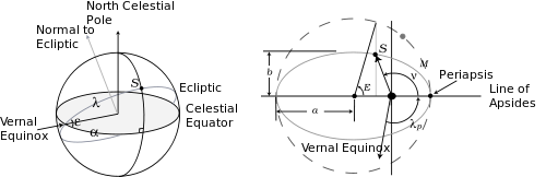
The celestial sphere and the Sun’s elliptical orbit as seen by a geocentric observer looking normal to the ecliptic showing the 6 angles (M, λp, α, ν, λ, E) needed for the calculation of the equation of time. For the sake of clarity the drawings are not to scale.
All these angles are shown in the figure on the right, which shows the celestial sphere and the Sun’s elliptical orbit seen from the Earth (the same as the Earth’s orbit seen from the Sun). In this figure ε is the obliquity, while e = √1 − (b/a)2 is the eccentricity of the ellipse.
Now given a value of 0 ≤ M ≤ 2π, one can calculate α(M) by means of the following well-known procedure:[27]: 89
First, given M, calculate E from Kepler’s equation:[31]: 159

Although this equation cannot be solved exactly in closed form, values of E(M) can be obtained from infinite (power or trigonometric) series, graphical, or numerical methods. Alternatively, note that for e = 0, E = M, and by iteration:[32]: 2

This approximation can be improved, for small e, by iterating again,
- ,

and continued iteration produces successively higher order terms of the power series expansion in e. For small values of e (much less than 1) two or three terms of the series give a good approximation for E; the smaller e, the better the approximation.
Next, knowing E, calculate the true anomaly ν from an elliptical orbit relation[31]: 165

The correct branch of the multiple valued function arctan x to use is the one that makes ν a continuous function of E(M) starting from νE=0 = 0. Thus for 0 ≤ E < π use arctan x = arctan x, and for π < E ≤ 2π use arctan x = arctan x + π. At the specific value E = π for which the argument of tan is infinite, use ν = E. Here arctan x is the principal branch, |arctan x| < π/2; the function that is returned by calculators and computer applications. Alternatively, this function can be expressed in terms of its Taylor series in e, the first three terms of which are:
- .

For small e this approximation (or even just the first two terms) is a good one. Combining the approximation for E(M) with this one for ν(E) produces
- .

The relation ν(M) is called the equation of the center; the expression written here is a second-order approximation in e. For the small value of e that characterises the Earth’s orbit this gives a very good approximation for ν(M).
Next, knowing ν, calculate λ from its definition:

The value of λ varies non-linearly with M because the orbit is elliptical and not circular. From the approximation for ν:
- .

Finally, knowing λ calculate α from a relation for the right triangle on the celestial sphere shown above[33]: 22

Note that the quadrant of α is the same as that of λ, therefore reduce λ to the range 0 to 2π and write
- ,

where k is 0 if λ is in quadrant 1, it is 1 if λ is in quadrants 2 or 3 and it is 2 if λ is in quadrant 4. For the values at which tan is infinite, α = λ.
Although approximate values for α can be obtained from truncated Taylor series like those for ν,[34]: 32 it is more efficacious to use the equation[35]: 374

where y = tan2(ε/2). Note that for ε = y = 0, α = λ and iterating twice:
- .

Equation of time[edit]
The equation of time is obtained by substituting the result of the right ascension calculation into an equation of time formula. Here Δt(M) = M + λp − α[λ(M)] is used; in part because small corrections (of the order of 1 second), that would justify using E, are not included, and in part because the goal is to obtain a simple analytical expression. Using two-term approximations for λ(M) and α(λ) allows Δt to be written as an explicit expression of two terms, which is designated Δtey because it is a first order approximation in e and in y.
- minutes

This equation was first derived by Milne,[35]: 375 who wrote it in terms of λ = M + λp. The numerical values written here result from using the orbital parameter values, e = 0.016709, ε = 23.4393° = 0.409093 radians, and λp = 282.9381° = 4.938201 radians that correspond to the epoch 1 January 2000 at 12 noon UT1. When evaluating the numerical expression for Δtey as given above, a calculator must be in radian mode to obtain correct values because the value of 2λp − 2π in the argument of the second term is written there in radians. Higher order approximations can also be written,[36]: Eqs (45) and (46) but they necessarily have more terms. For example, the second order approximation in both e and y consists of five terms[28]: 1535

This approximation has the potential for high accuracy, however, in order to achieve it over a wide range of years, the parameters e, ε, and λp must be allowed to vary with time.[27]: 86 [28]: 1531,1535 This creates additional calculational complications. Other approximations have been proposed, for example, Δte[27]: 86 [37] which uses the first order equation of the center but no other approximation to determine α, and Δte2[38] which uses the second order equation of the center.
The time variable, M, can be written either in terms of n, the number of days past perihelion, or D, the number of days past a specific date and time (epoch):
- days days


Here MD is the value of M at the chosen date and time. For the values given here, in radians, MD is that measured for the actual Sun at the epoch, 1 January 2000 at 12 noon UT1, and D is the number of days past that epoch. At periapsis M = 2π, so solving gives D = Dp = 2.508109. This puts the periapsis on 4 January 2000 at 00:11:41 while the actual periapsis is, according to results from the Multiyear Interactive Computer Almanac[39] (abbreviated as MICA), on 3 January 2000 at 05:17:30. This large discrepancy happens because the difference between the orbital radius at the two locations is only 1 part in a million; in other words, radius is a very weak function of time near periapsis. As a practical matter this means that one cannot get a highly accurate result for the equation of time by using n and adding the actual periapsis date for a given year. However, high accuracy can be achieved by using the formulation in terms of D.

Curves of Δt and Δtey along with symbols locating the daily values at noon (at 10-day intervals) obtained from the Multiyear Interactive Computer Almanac vs d for the year 2000
When D > Dp, M is greater than 2π and one must subtract a multiple of 2π (that depends on the year) from it to bring it into the range 0 to 2π. Likewise for years prior to 2000 one must add multiples of 2π. For example, for the year 2010, D varies from 3653 on 1 January at noon to 4017 on 31 December at noon; the corresponding M values are 69.0789468 and 75.3404748 and are reduced to the range 0 to 2π by subtracting 10 and 11 times 2π respectively. One can always write D = nY + d, where nY is the number of days from the epoch to noon on 1 January of the desired year, and 0 ≤ d ≤ 364 (365 if the calculation is for a leap year).
The result of the computations is usually given as either a set of tabular values, or a graph of the equation of time as a function of d. A comparison of plots of Δt, Δtey, and results from MICA all for the year 2000 is shown in the figure on the right. The plot of Δtey is seen to be close to the results produced by MICA, the absolute error, Err = |Δtey − MICA2000|, is less than 1 minute throughout the year; its largest value is 43.2 seconds and occurs on day 276 (3 October). The plot of Δt is indistinguishable from the results of MICA, the largest absolute error between the two is 2.46 s on day 324 (20 November).
[edit]
For the choice of the appropriate branch of the arctan relation with respect to function continuity a modified version of the arctangent function is helpful. It brings in previous knowledge about the expected value by a parameter. The modified arctangent function is defined as:
- .

It produces a value that is as close to η as possible. The function round rounds to the nearest integer.
Applying this yields:
- .

The parameter M + λp arranges here to set Δt to the zero nearest value which is the desired one.
Secular effects[edit]
The difference between the MICA and Δt results was checked every 5 years over the range from 1960 to 2040. In every instance the maximum absolute error was less than 3 s; the largest difference, 2.91 s, occurred on 22 May 1965 (day 141). However, in order to achieve this level of accuracy over this range of years it is necessary to account for the secular change in the orbital parameters with time. The equations that describe this variation are:[27]: 86 [28]: 1531,1535

According to these relations, in 100 years (D = 36525), λp increases by about 0.5% (1.7°), e decreases by about 0.25%, and ε decreases by about 0.05%.
As a result, the number of calculations required for any of the higher-order approximations of the equation of time requires a computer to complete them, if one wants to achieve their inherent accuracy over a wide range of time. In this event it is no more difficult to evaluate Δt using a computer than any of its approximations.
In all this note that Δtey as written above is easy to evaluate, even with a calculator, is accurate enough (better than 1 minute over the 80-year range) for correcting sundials, and has the nice physical explanation as the sum of two terms, one due to obliquity and the other to eccentricity that was used previously in the article. This is not true either for Δt considered as a function of M or for any of its higher-order approximations.
Alternative calculation[edit]
Another procedure for calculating the equation of time can be done as follows.[37] Angles are in degrees; the conventional order of operations applies.
- n = 360°/365.24 days,
where n is the Earth’s mean angular orbital velocity in degrees per day, a.k.a. «the mean daily motion».

where D is the date, counted in days starting at 1 on 1 January (i.e. the days part of the ordinal date in the year). 9 is the approximate number of days from the December solstice to 31 December. A is the angle the Earth would move on its orbit at its average speed from the December solstice to date D.

B is the angle the Earth moves from the solstice to date D, including a first-order correction for the Earth’s orbital eccentricity, 0.0167 . The number 3 is the approximate number of days from 31 December to the current date of the Earth’s perihelion. This expression for B can be simplified by combining constants to:
- .


Here, C is the difference between the angle moved at mean speed, and at the angle at the corrected speed projected onto the equatorial plane, and divided by 180° to get the difference in «half-turns». The value 23.44° is the tilt of the Earth’s axis («obliquity»). The subtraction gives the conventional sign to the equation of time. For any given value of x, arctan x (sometimes written as tan−1 x) has multiple values, differing from each other by integer numbers of half turns. The value generated by a calculator or computer may not be the appropriate one for this calculation. This may cause C to be wrong by an integer number of half-turns. The excess half-turns are removed in the next step of the calculation to give the equation of time:
- minutes

The expression nint(C) means the nearest integer to C. On a computer, it can be programmed, for example, as INT(C + 0.5). Its value is 0, 1, or 2 at different times of the year. Subtracting it leaves a small positive or negative fractional number of half turns, which is multiplied by 720, the number of minutes (12 hours) that the Earth takes to rotate one half turn relative to the Sun, to get the equation of time.
Compared with published values,[8] this calculation has a root mean square error of only 3.7 s. The greatest error is 6.0 s. This is much more accurate than the approximation described above, but not as accurate as the elaborate calculation.
Addendum about solar declination[edit]
The value of B in the above calculation is an accurate value for the Sun’s ecliptic longitude (shifted by 90°), so the solar declination δ becomes readily available:

which is accurate to within a fraction of a degree.
See also[edit]
- Azimuth
- Milankovitch cycles
Notes and footnotes[edit]
- Notes
- ^ As an example of the inexactness of the dates, according to the U.S. Naval Observatory’s Multiyear Interactive Computer Almanac the equation of time was zero at 02:00 UT1 on 16 April 2011.
- ^ equalization (adjustment)
- ^ This meant that any clock being set to mean time by Huygens’s tables was consistently about 15 minutes slow compared to today’s mean time.
- ^ See above
- ^ See barycentre
- ^ Universal Time is discontinuous at mean midnight so another quantity day number N, an integer, is required in order to form the continuous quantity time t: t = N + UT/24 hr days.
- Footnotes
- ^ a b Maskelyne, Nevil (1767). The Nautical Almanac and Astronomical Ephemeris. London: Commissioners of Longitude.
- ^ Milham, Willis I. (1945). Time and Timekeepers. New York: Macmillan. pp. 11–15. ISBN 978-0780800083.
- ^ British Commission on Longitude (1794). Nautical Almanac and Astronomical Ephemeris for the year 1803. London, UK: C. Bucton.
- ^ a b Heilbron, J. L. (1999). The Sun in the Church: Cathedrals as Solar Observatories. Cambridge, MA: Harvard University Press. ISBN 9780674005365.
- ^ a b Jenkins, Alejandro (2013). «The Sun’s position in the sky». European Journal of Physics. 34 (3): 633–652. arXiv:1208.1043. Bibcode:2013EJPh…34..633J. doi:10.1088/0143-0807/34/3/633. S2CID 119282288.
- ^ Astronomical Applications Department. «The Equation of Time». United States Naval Observatory. United States Navy. Retrieved 1 August 2022.
- ^ Astronomical Applications Department. «Astronomical Almanac Glossary». United States Naval Observatory. United States Navy. Retrieved 1 August 2022.
- ^ a b c Waugh, Albert E. (1973). Sundials, Their Theory and Construction. New York: Dover Publications. p. 205. ISBN 978-0-486-22947-8.
- ^ Kepler, Johannes (1995). Epitome of Copernican Astronomy & Harmonies of the World. Prometheus Books. ISBN 978-1-57392-036-0.
- ^ McCarthy & Seidelmann 2009, p. 9.
- ^ Neugebauer, Otto (1975), A History of Ancient Mathematical Astronomy, Studies in the History of Mathematics and Physical Sciences, vol. 1, New York / Heidelberg / Berlin: Springer-Verlag, pp. 984–986, doi:10.1007/978-3-642-61910-6, ISBN 978-0-387-06995-1
- ^ Toomer, G.J. (1998). Ptolemy’s Almagest. Princeton University Press. p. 171. ISBN 978-0-691-00260-6.
- ^ Kennedy, E. S. (1956). «A Survey of Islamic Astronomical Tables». Transactions of the American Philosophical Society. 46 (2): 141. doi:10.2307/1005726. hdl:2027/mdp.39076006359272. JSTOR 1005726.
Reprinted in: Kennedy, E. S. (1989). A survey of Islamic astronomical tables (2nd ed.). Philadelphia, PA: American Philosophical Society. p. 19. ISBN 9780871694621. - ^ Olmstead, Dennison (1866). A Compendium of Astronomy. New York: Collins & Brother.
- ^ a b Huygens, Christiaan (1665). Kort Onderwys aengaende het gebruyck der Horologien tot het vinden der Lenghten van Oost en West. The Hague: [publisher unknown].
- ^ Flamsteed, John (1673) [1672 for the imprint, and bound with other sections printed 1673]. De Inaequalitate Dierum Solarium. London: William Godbid.
- ^ Vince, S. «A Complete System of Astronomy». 2nd edition, volume 1, 1814
- ^ Mills, Allan (2007). «Robert Hooke’s ‘universal joint’ and its application to sundials and the sundial-clock». Notes Rec. R. Soc. Royal Society Publishing. 61 (2): 219–236. doi:10.1098/rsnr.2006.0172.
- ^ Maskelyne, Nevil (1764). «Some Remarks upon the Equation of Time, and the True Manner of Computing It». Philosophical Transactions. Royal Society. 54: 336–347. JSTOR 105569.
- ^ a b «The Equation of Time». Royal Museums Greenwich. Archived from the original on 10 September 2015. Retrieved 29 January 2021.
- ^ «Eccentricity». Analemma. Retrieved 29 January 2021.
- ^ a b Taylor, Kieran (4 November 2018). «The Equation of Time: Why Sundial time Differs From Clock Time Depending On Time Of Year». moonkmft. Retrieved 29 January 2021.
- ^ «Obliquity». Analemma. Retrieved 29 January 2021.
- ^ Karney, Kevin (December 2005). «Variation in the Equation of Time» (PDF).
- ^ Meeus 1997.
- ^ «How to find the exact time of solar noon, wherever you are in the world». Spot-On Sundials. London. Retrieved 23 July 2013.
- ^ a b c d e Duffett-Smith, Peter; Zwart, Jonathan (2017). Practical astronomy with your calculator or spreadsheet (4th ed.). Cambridge, UK: Cambridge University Press. ISBN 9781108436076.
- ^ a b c d e f Hughes, David W.; Yallop, B. D.; Hohenkerk, C. Y. (June 1989). «The Equation of Time». Monthly Notices of the Royal Astronomical Society. 238 (4): 1529–1535. doi:10.1093/mnras/238.4.1529. ISSN 0035-8711.
- ^ a b Astronomical Applications Department. «Computing Approximate Sidereal Time». United States Naval Observatory. United States Navy. Retrieved 1 August 2022.
- ^ Roy, A. E. (1988). Orbital motion (3rd ed.). Bristol, England: A. Hilger. ISBN 0-85274-228-2.
- ^ a b Moulton, Forest Ray (1914). An introduction to celestial mechanics (2nd ed.). Macmillan.
- ^ Hinch, E. J. (2002). Perturbation methods. Cambridge, UK: Cambridge University Press. doi:10.1017/CBO9781139172189. ISBN 9781139172189.
- ^ Burington, Richard S. (1965) [1933]. Handbook of Mathematical Tables and Formulas (4th ed.). McGraw-Hill. LCCN 63-23531.
- ^ Whitman, Alan M (2007). «A Simple Expression for the Equation of Time». Compendium. North American Sundial Society. 14: 29–33. CiteSeerX 10.1.1.558.1314. ISSN 1074-8059.
- ^ a b Milne, R. M. (December 1921). «Note on the Equation of Time». The Mathematical Gazette. Mathematical Association. 10 (155): 372–375. doi:10.1017/S0025557200232944. S2CID 126276982.
- ^ Müller, M. (1995). «Equation of Time: Problem in Astronomy» (PDF). Acta Physica Polonica A. Institute of Physics, Polish Academy of Sciences. 88 (Supplement): S49–S67.
- ^ a b Williams, David O. (2009). «The Latitude and Longitude of the Sun». Archived from the original on 23 March 2012.
- ^ «Approximate Solar Coordinates», «Naval Oceanography Portal».
- ^ United States Naval Observatory April 2010, Multiyear Interactive Computer Almanac (version 2.2.1), Richmond VA: Willmann-Bell.
References[edit]
- Helyar, A.G. «Sun Data». Archived from the original on 11 January 2004.
- Meeus, J (1997). Mathematical Astronomy Morsels. Richmond, Virginia: Willman-Bell.
{{cite book}}: CS1 maint: ref duplicates default (link) - McCarthy, Dennis D.; Seidelmann, P. Kenneth (2009). TIME From Earth Rotation to Atomic Physics. Weinheim: Wiley VCH. ISBN 978-3-527-40780-4.
{{cite book}}: CS1 maint: ref duplicates default (link)
External links[edit]
- NOAA Solar Calculator
- USNO data services Archived 29 May 2014 at the Wayback Machine (include rise/set/transit times of the Sun and other celestial objects)
- The equation of time described on the Royal Greenwich Observatory web site
- The Equation of Time and the Analemma, by Kieron Taylor
- An article by Brian Tung containing a link to a C program using a more accurate formula than most (particularly at high inclinations and eccentricities). The program can calculate solar declination, Equation of Time, or Analemma.
- Doing calculations using Ptolemy’s geocentric planetary models with a discussion of his E.T. graph
- Equation of Time Longcase Clock by John Topping C.1720
- The equation of time correction-table A page describing how to correct a clock to a sundial.
- Solar tempometer – Calculate your solar time, including the equation of time.
Уравнение времени и связь среднего и истинного времени.
Уравнением
времени
называется разность среднего и истинного
времени, численно равная разности
часовых углов среднего и истинного
Солнца, т.е.
![]() =
=
t![]()
— t![]()
(2.3)
или
![]() =
=![]()
![]() —
—![]()
![]()
Уравнение
времени можно выбрать из МАЕ или с
графика. Из графика видно, что четыре
раза в году уравнение времени равно
нулю (16 апреля, 14 июня, 1 сентября и 25
декабря) и четыре экстремальных значения:
(11 февраля +14,3м,
15 мая -3,8м,
26 июля +6,4м
и 3 ноября -16,4м).
Эти знания помогли героям романа Жюль
Верна «Таинственный остров»
определить долготу своего местонахождения.
Уравнение
времени устанавливает взаимосвязь
между истинным и средним временем, на
основании которой можно решать следующие
задачи.
-
Получение
часового угла Солнца по известному
времени.

t![]() = T ± 12 —
= T ± 12 —![]()
-
Получение
времени кульминации Солнца.
Для
верхней кульминации t = 0, поэтому из последней формулы имеем
Тв.к
= 12ч
+
![]()
Эту
взаимосвязь наглядно можно увидеть на
представленном фрагменте МАЕ (внизу на
правом развороте ежедневных страниц).
Связь среднего и звездного времени.
Применяя
основную формулу времени к среднему
Солнцу S = t![]() +
+![]()
![]() ,
,
но из формулы времени t![]() = T ± 12ч,
= T ± 12ч,
поэтому
S
= T ± 12ч
+
![]()
![]()
Времена на различных меридианах, местное время.
Изобразим
небесную сферу в проекции на небесный
экватор.
Местное
среднее время (Тм)
—
это промежуток времени между моментом
нижней кульминации среднего Солнца и
текущим моментов времени для наблюдателя,
находящегося на меридиане с долготой
![]() .Гринвичское
.Гринвичское
время (Тгр)
— это местное время гринвичского
меридиана.
Из рисунка видно, что на
востоке местное время (Тм)
всегда больше гринвичского времени
(Тгр)
на величину дуги долготы
![]()
Тгр
= Тм
±![]() WE
WE
Тм
= Тгр
±![]() EW
EW
(2.5)
Гринвичское
время иногда называют всемирным. Оно
является аргументом для входа в Морской
астрономический ежегодник (МАЕ).
Местное
время Тм
на практике не используется по двум
причинам:
-
Судно
движется, поэтому долгота судна
изменяется, что создает трудности в
расчете местного времени. -
На
суше для двух наблюдателей, имеющих
разность долгот

 °,
°,
местные времена будут отличаться на
величинуТм
= 15
°.

Поясное время.
Широкое
распространение получила система
поясного времени,
принятая на астрономическом конгрессе
1884 г по предложению канадского инженера
транспорта Флеминга.
Вся Земля
разделена на 24 часовых пояса по 15° (или
1ч)
долготы в каждом. Меридианы 0°, 15°, 30° и
далее через 15° (до 180°) являются центральными
для каждого пояса, меридианы с долготами
7°30′, 22°30′ и далее — это границы поясов.
Они точно следуют по меридианам только
в открытом море и океане.
Поясным
временем Тп
называется местное время центрального
меридиана данного часового пояса,
принятое по всей территории пояса.
Пояс
с центральным меридианом Гринвича
считается нулевым, а от него идет
нумерация поясов к E или W, до двенадцатого
пояса включительно.

Для
определения номера пояса,
в котором находится судно или данный
пункт, надо его долготу разделить на
15°. Частное от деления дает номер пояса,
а если в остатке получится больше 7°30′,
то рассчитанный таким образом номер
пояса увеличивается на единицу.
Примеры:
![]() =
=
20°Е, № = 1Е![]() =
=
28W°Е, № = 2W
Свойства
поясного времени:
-
поясное
время в соседних поясах отличается
ровно на 1ч; -
разница
поясного времени в любых двух часовых
поясах равна разности их номеров; -
поясное
время любого пояса отличается от
гринвичского, т.е. от времени нулевого
пояса, на величину номера пояса:
Тп
= Тгр
± ТEW
Тгр
= Тп
± ТWE
(2.6)
Местное
время в пределах одного часового пояса
теоретически не должно отличаться от
поясного Тп
более чем на 30м,
что соответствует ширине пояса в
7°30′.
Однако, на суше границы часовых
поясов не всегда совпадают с меридианами,
кратными по долготе 7°30′. Они устанавливаются
правительством стран и обычно совпадают
с государственными, административными
или географическими границами. Границы
указаны на карте №90080.

![]()
График уравнения времени (синяя линия) и двух его составляющих при определении этого уравнения как УВ = ССВ — ИСВ.

![]()
Уравнение времени (по «инвертированному» определению, принятому в англоязычной литературе). График выше нуля — солнечные часы «спешат», ниже нуля — солнечные часы «отстают»
Уравнение времени — разница между средним солнечным временем (ССВ) и истинным солнечным временем (ИСВ), то есть УВ = ССВ — ИСВ[1]. Эта разница в каждый конкретный момент времени одинакова для наблюдателя в любой точке Земли. Уравнение времени можно узнать из специализированных астрономических изданий, астрономических программ или вычислить по формуле, приведенной ниже.
В таких изданиях, как «Астрономический календарь», уравнение времени определяется как разность часовых углов среднего экваториального солнца и истинного солнца, то есть, при таком определении УВ = ССВ — ИСВ[2].
В англоязычных изданиях часто применяется иное определение уравнения времени (т.н. «инвертированное»): УВ = ИСВ — ССВ, то есть разница между истинным солнечным временем (ИСВ) и средним солнечным временем (ССВ).
Содержание
- 1 Некоторые пояснения к определению
- 2 Объяснение неравномерности движения истинного Солнца
- 2.1 Неравномерность, обусловленная эллиптичностью орбиты
- 2.2 Неравномерность обусловленная наклоном земной оси
- 2.3 Уравнение времени как сумма обеих неравномерностей
- 3 Расчёт
- 4 Примечания
- 5 Ссылки
Некоторые пояснения к определению
Можно встретить определение уравнения времени как разницы «местного истинного солнечного времени» и «местного среднего солнечного времени» (в англоязычной литературе — local apparent solar time и local mean solar time). Данное определение формально более точно, но не влияет на результат, так как для любой конкретной точки на Земле эта разница одинакова.
Кроме того, не следует путать ни «местное истинное солнечное время», ни «местное среднее солнечное время» с поясным временем — временем «официальных» часов (например, «Московское время»).
Объяснение неравномерности движения истинного Солнца
В отличие от звезд, чьё видимое суточное движение практически равномерно и обусловлено только вращением Земли вокруг своей оси, суточное движение Солнца не равномерно, так как обусловлено и вращением Земли вокруг своей оси, и вращением Земли вокруг Солнца, и наклоном земной оси к плоскости эклиптики.
Неравномерность, обусловленная эллиптичностью орбиты
Вращение Земли вокруг Солнца происходит по эллиптической орбите. Согласно второму закону Кеплера, такое движение неравномерно, оно быстрее в области перигелия и медленнее в области афелия. Для наблюдателя, находящегося на Земле, это выражается в том, что видимое движение Солнца по эклиптике относительно неподвижных звезд то ускоряется, то замедляется.
Неравномерность обусловленная наклоном земной оси
Поскольку плоскость эклиптики наклонена к плоскости небесного экватора, имеет место следующее явление:
- Солнце вблизи солнцестояний (зимнего и летнего) движется почти параллельно к небесному экватору, и скорость его перемещения практически полностью вычитается из суточного движения небесной сферы — результирующая скорость изменения часового угла Солнца минимальна;
- Солнце вблизи равноденствий (осеннего и весеннего) движется под максимальным углом к небесному экватору, и скорость его перемещения лишь частично вычитается из суточного движения небесной сферы — результирующая скорость изменения часового угла Солнца максимальна.
Уравнение времени как сумма обеих неравномерностей

![]()
1. Влияние эксцентриситета 2. Влияние наклона эклиптики 3. Сумма — Уравнение времени 4. Позиция истинного Солнца относительно среднего Солнца.
(Графики приведены в соответствии с «инвертированным» определением уравнения времени, принятым в англоязычной литературе)
Кривая уравнения времени является суммой двух периодических кривых — с периодами 1 год и 6 месяцев. Практически синусоидальная кривая с годичным периодом обусловлена неравномерным движением Солнца по эклиптике. Эта часть уравнения времени называется уравнением центра или уравнением от эксцентриситета. Синусоида с периодом 6 месяцев представляет разность времён, вызванную наклоном эклиптики к небесному экватору и называется уравнением от наклона эклиптики[1].
Уравнение времени обращается в ноль четыре раза в году: 14 апреля, 14 июня, 2 сентября и 24 декабря.
Соответственно, в каждое время года существует свой максимум уравнения времени: около 12 февраля — +14,3 мин, 15 мая — −3,8 мин, 27 июля — +6,4 мин и 4 ноября — −16,4 мин. Точные величины уравнения времени даются в астрономических ежегодниках.
Может применяться как дополнительная функция в некоторых моделях часов.
Расчёт
Уравнение можно аппроксимировать отрезком ряда Фурье как сумму двух синусоидальных кривых с периодами, соответственно, на один год и шесть месяцев:

где
- если углы выражаются в градусах.
 если углы выражаются в градусах.
или
- если углы выражаются в радианах.
 если углы выражаются в радианах.
- Там, где — количество дней, например:
 — количество дней, например:
- на 1 января
 на 1 января
- на 2 января
 на 2 января
и так далее.
Примечания
- ↑ 1 2 Кононович Э. В., Мороз В. И. «Общий курс астрономии» Учебное пособие под ред. В. В. Иванова. Изд. 2-е, испр. М.: Едиториал УРСС, 2004. — 544 с. ISBN 5-354-0866-2, 3000 экз.
- ↑ Астрономический календарь. Постоянная часть / Ответственный редактор Абалакин В.К.. — 7-е изд. — М.: Наука, 1981. — С. 19.
Ссылки
- Величина колебаний уравнения времени в течение года на портале Гринвичской королевской обсерватории.
- Уравнение времени на сегодняшний день — визуализация.
- Образец построения графика уравнения времени, где прорисованы:
- 1 — составляющая уравнения времени, определяемая неравномерностью движения Земли по орбите,
- 2 — составляющая уравнения времени, определяемая наклоном эклиптики к экватору,
- 3 — уравнение времени.