Как найти матричное исчисление матрицы - Avtoru.top

Метод матричного исчисления

Дана система линейных уравнений

x₁-4x₂-2x₃=-3

3x₁+x₂+x₃=5

-3x₁-5x₂-6x₃=-7

Доказать ее совместимость и решить двумя способами:

Решение:

найдем решение задачи, методом матричного исчисления.

Чтобы записать ее виде матричного уравнения и решить это матричное уравнение, используем правила действия над матрицами.

Для этого введем обозначения:

Далее, система записывается в виде следующего уравнения , откуда следует, что . Найдем обратную матрицу для матрицы А. Посчитаем сначала алгебраические дополнения для элементов матрицы А.

, ,,

Найдем определитель .

По формуле для отыскания обратной матрицы имеем

Найдем матрицу строку Х, которая и даст решение системы

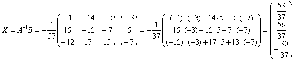
х1=53/37; х2=56/37; х3=-30/37

Ответ прост!

————————————————————————————————-
Решение задач численные методы. Заказать подобную работу!

————————————————————————————————-
Калькулятор матричного исчисления онлайн

13,149 total views, 2 views today

Источник

Решение матричных уравнений

Финальная глава саги.

Линейная алгебра и, в частности, матрицы — это основа математики нейросетей. Когда говорят «машинное обучение», на самом деле говорят «перемножение матриц», «решение матричных уравнений» и «поиск коэффициентов в матричных уравнениях».

Понятно, что между простой матрицей в линейной алгебре и нейросетью, которая генерирует котов, много слоёв усложнений, дополнительной логики, обучения и т. д. Но здесь мы говорим именно о фундаменте. Цель — чтобы стало понятно, из чего оно сделано.

Краткое содержание прошлых частей:

Линейная алгебра изучает векторы, матрицы и другие понятия, которые относятся к упорядоченным наборам данных. Линейной алгебре интересно, как можно трансформировать эти упорядоченные данные, складывать и умножать, всячески обсчитывать и находить в них закономерности.
Вектор — это набор упорядоченных данных в одном измерении. Можно упрощённо сказать, что это последовательность чисел.
Матрица — это тоже набор упорядоченных данных, только уже не в одном измерении, а в двух (или даже больше).
Матрицу можно представить как упорядоченную сумку с данными. И с этой сумкой как с единым целым можно совершать какие-то действия. Например, делить, умножать, менять знаки.
Матрицы можно складывать и умножать на другие матрицы. Это как взять две сумки с данными и получить третью сумку, тоже с данными, только теперь какими-то новыми.
Матрицы перемножаются по довольно замороченному алгоритму. Арифметика простая, а порядок перемножения довольно запутанный.

И вот наконец мы здесь: если мы можем перемножать матрицы, то мы можем и решить матричное уравнение.

❌ Никакого практического применения следующего материала в народном хозяйстве вы не увидите. Это чистая алгебра в несколько упрощённом виде. Отсюда до практики далёкий путь, поэтому, если нужно что-то практическое, — посмотрите, как мы генерим Чехова на цепях Маркова.

Что такое матричное уравнение

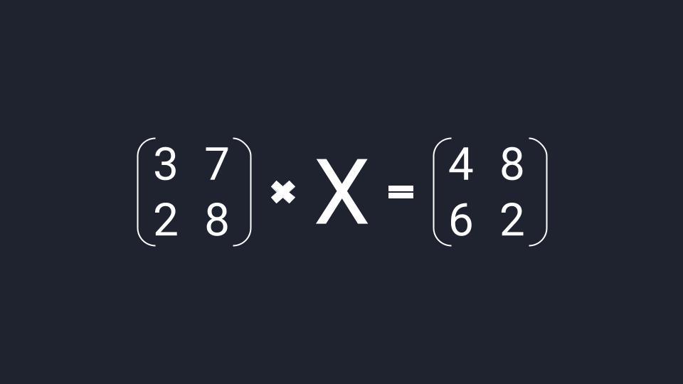
Матричное уравнение — это когда мы умножаем известную матрицу на матрицу Х и получаем новую матрицу. Наша задача — найти неизвестную матрицу Х.

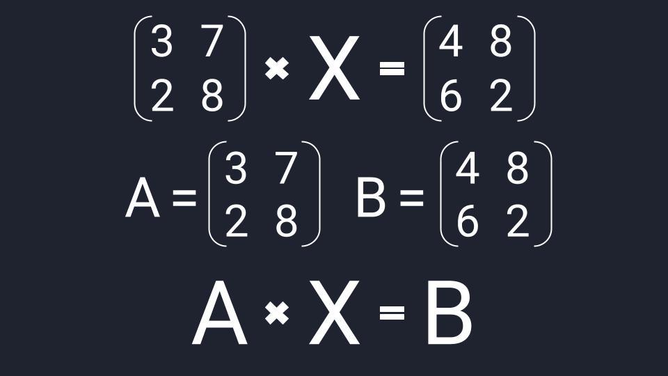
Шаг 1. Упрощаем уравнение

Вместо известных числовых матриц вводим в уравнение буквы: первую матрицу обозначаем буквой A, вторую — буквой B. Неизвестную матрицу X оставляем. Это упрощение поможет составить формулу и выразить X через известную матрицу.

Приводим матричное уравнение к упрощённому виду

Шаг 2. Вводим единичную матрицу

В линейной алгебре есть два вспомогательных понятия: обратная матрица и единичная матрица. Единичная матрица состоит из нулей, а по диагонали у неё единицы. Обратная матрица — это такая, которая при умножении на исходную даёт единичную матрицу.

Можно представить, что есть число 100 — это «сто в первой степени», 100 1

И есть число 0,01 — это «сто в минус первой степени», 100 -1

При перемножении этих двух чисел получится единица:
100 1 × 100 -1 = 100 × 0,01 = 1.

Вот такое, только в мире матриц.

Зная свойства единичных и обратных матриц, делаем алгебраическое колдунство. Умножаем обе известные матрицы на обратную матрицу А -1 . Неизвестную матрицу Х оставляем без изменений и переписываем уравнение:

А -1 × А × Х = А -1 × В

Добавляем единичную матрицу и упрощаем запись:

А -1 × А = E — единичная матрица

E × Х = А -1 × В — единичная матрица, умноженная на исходную матрицу, даёт исходную матрицу. Единичную матрицу убираем

Х = А -1 × В — новая запись уравнения

После введения единичной матрицы мы нашли способ выражения неизвестной матрицы X через известные матрицы A и B.

💡 Смотрите, что произошло: раньше нам нужно было найти неизвестную матрицу. А теперь мы точно знаем, как её найти: нужно рассчитать обратную матрицу A -1 и умножить её на известную матрицу B. И то и другое — замороченные процедуры, но с точки зрения арифметики — просто.

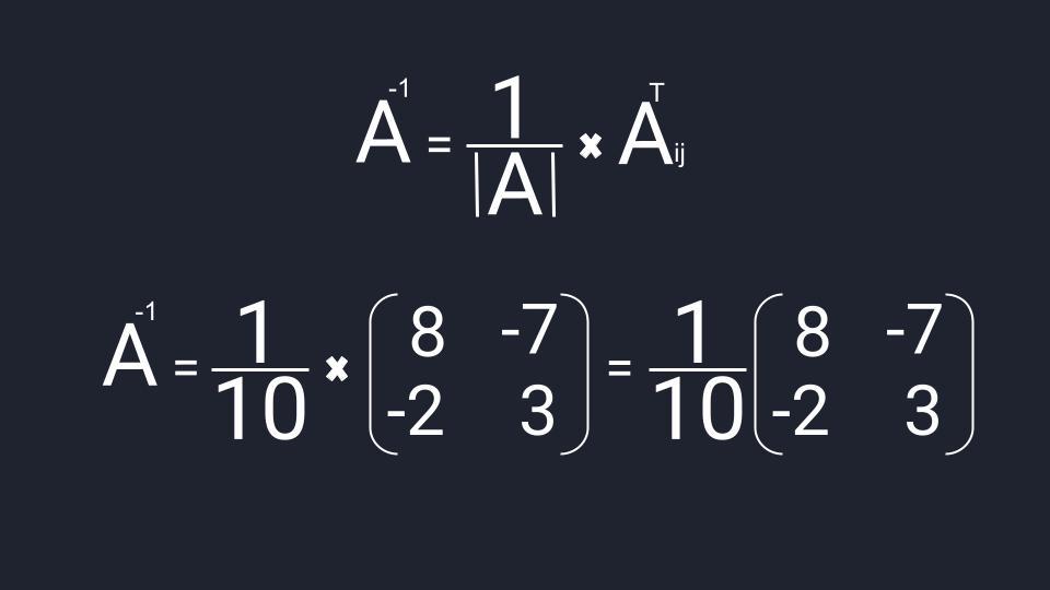
Шаг 3. Находим обратную матрицу

Вспоминаем формулу и порядок расчёта обратной матрицы:

Делим единицу на определитель матрицы A.
Считаем транспонированную матрицу алгебраических дополнений.
Перемножаем значения и получаем нужную матрицу.

Собираем формулу и получаем обратную матрицу. Для удобства умышленно оставляем перед матрицей дробное число, чтобы было проще считать.

Третье действие: получаем обратную матрицу

Шаг 4. Вычисляем неизвестную матрицу

Нам остаётся посчитать матрицу X: умножаем обратную матрицу А -1 на матрицу B. Дробь держим за скобками и вносим в матрицу только при условии, что элементы новой матрицы будут кратны десяти — их можно умножить на дробь и получить целое число. Если кратных элементов не будет — дробь оставим за скобками.

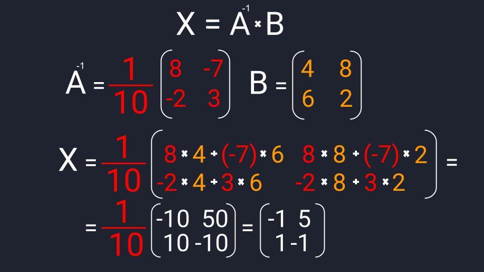Решаем матричное уравнение и находим неизвестную матрицу X. Мы получили кратные числа и внесли дробь в матрицу

Шаг 5. Проверяем уравнение

Мы решили матричное уравнение и получили красивый ответ с целыми числами. Выглядит правильно, но в случае с матрицами этого недостаточно. Чтобы проверить ответ, нам нужно вернуться к условию и умножить исходную матрицу A на матрицу X. В результате должна появиться матрица B. Если расчёты совпадут — мы всё сделали правильно. Если будут отличия — придётся решать заново.

👉 Часто начинающие математики пренебрегают финальной проверкой и считают её лишней тратой времени. Сегодня мы разобрали простое уравнение с двумя квадратными матрицами с четырьмя элементами в каждой. Когда элементов будет больше, в них легко запутаться и допустить ошибку.

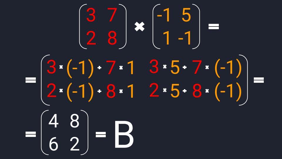Проверяем ответ и получаем матрицу B — наши расчёты верны

Ну и что

Алгоритм решения матричных уравнений несложный, если знать отдельные его компоненты. Дальше на основе этих компонентов математики переходят в более сложные пространства: работают с многомерными матрицами, решают более сложные уравнения, постепенно выходят на всё более и более абстрактные уровни. И дальше, в конце пути, появляется датасет из миллионов котиков. Этот датасет раскладывается на пиксели, каждый пиксель оцифровывается, цифры подставляются в матрицы, и уже огромный алгоритм в автоматическом режиме генерирует изображение нейрокотика:

Онлайн калькулятор. Решение систем линейных уравнений. Матричный метод. Метод обратной матрицы.

Используя этот онлайн калькулятор для решения систем линейных уравнений (СЛУ) матричным методом (методом обратной матрицы), вы сможете очень просто и быстро найти решение системы.

Воспользовавшись онлайн калькулятором для решения систем линейных уравнений матричным методом (методом обратной матрицы), вы получите детальное решение вашей задачи, которое позволит понять алгоритм решения задач на решения систем линейных уравнений, а также закрепить пройденный материал.

Решить систему линейных уравнений матричным методом

Изменить названия переменных в системе

Заполните систему линейных уравнений:

Ввод данных в калькулятор для решения систем линейных уравнений матричным методом

В онлайн калькулятор вводить можно числа или дроби. Более подробно читайте в правилах ввода чисел.
Для изменения в уравнении знаков с «+» на «-» вводите отрицательные числа.
Если в уравнение отсутствует какая-то переменная, то в соответствующем поле ввода калькулятора введите ноль.
Если в уравнение перед переменной отсутствуют числа, то в соответствующем поле ввода калькулятора введите единицу.

Например, линейное уравнение x ₁ — 7 x ₂ — x ₄ = 2

будет вводится в калькулятор следующим образом:

Дополнительные возможности калькулятора для решения систем линейных уравнений матричным методом

Между полями для ввода можно перемещаться нажимая клавиши «влево», «вправо», «вверх» и «вниз» на клавиатуре.
Вместо x ₁, x ₂, . вы можете ввести свои названия переменных.

Вводить можно числа или дроби (-2.4, 5/7, . ). Более подробно читайте в правилах ввода чисел.

Решение матричных уравнений: теория и примеры

Решение матричных уравнений: как это делается

Матричные уравнения имеют прямую аналогию с простыми алгебраическими уравнениями, в которых присутствует операция умножения. Например,

где x — неизвестное.

А, поскольку мы уже умеем находить произведение матриц, то можем приступать к рассмотрению аналогичных уравнений с матрицами, в которых буквы — это матрицы.

Итак, матричным уравнением называется уравнение вида

где A и B — известные матрицы, X — неизвестная матрица, которую требуется найти.

Как решить матричное уравнение в первом случае? Для того, чтобы решить матричное уравнение вида A ⋅ X = B , обе его части следует умножить на обратную к A матрицу слева:

По определению обратной матрицы, произведение обратной матрицы на данную исходную матрицу равно единичной матрице: , поэтому

Так как E — единичная матрица, то E ⋅ X = X . В результате получим, что неизвестная матрица X равна произведению матрицы, обратной к матрице A , слева, на матрицу B :

Как решить матричное уравнение во втором случае? Если дано уравнение

то есть такое, в котором в произведении неизвестной матрицы X и известной матрицы A матрица A находится справа, то нужно действовать аналогично, но меняя направление умножения на матрицу, обратную матрице A , и умножать матрицу B на неё справа:

Как видим, очень важно, с какой стороны умножать на обратную матрицу, так как . Обратная к A матрица умножается на матрицу B с той стороны, с которой матрица A умножается на неизвестную матрицу X . То есть с той стороны, где в произведении с неизвестной матрицей находится матрица A .

Как решить матричное уравнение в третьем случае? Встречаются случаи, когда в левой части уравнения неизвестная матрица X находится в середине произведения трёх матриц. Тогда известную матрицу из правой части уравнения следует умножить слева на матрицу, обратную той, которая в упомянутом выше произведении трёх матриц была слева, и справа на матрицу, обратную той матрице, которая располагалась справа. Таким образом, решением матричного уравнения

Решение матричных уравнений: примеры

Пример 1. Решить матричное уравнение

Решение. Данное уравнение имеет вид A ⋅ X = B , то есть в произведении матрицы A и неизвестной матрицы X матрица A находится слева. Поэтому решение следует искать в виде , то есть неизвестная матрица равна произведению матрицы B на матрицу, обратную матрице A слева. Найдём матрицу, обратную матрице A .

Сначала найдём определитель матрицы A :

Найдём алгебраические дополнения матрицы A :

Составим матрицу алгебраических дополнений:

Транспонируя матрицу алгебраических дополнений, находим матрицу, союзную с матрицей A :

Теперь у нас есть всё, чтобы найти матрицу, обратную матрице A :

Наконец, находим неизвестную матрицу:

Пример 2. Решить матричное уравнение

Пример 3. Решить матричное уравнение

Решение. Данное уравнение имеет вид X ⋅ A = B , то есть в произведении матрицы A и неизвестной матрицы X матрица A находится справа. Поэтому решение следует искать в виде , то есть неизвестная матрица равна произведению матрицы B на матрицу, обратную матрице A справа. Найдём матрицу, обратную матрице A .

Сначала найдём определитель матрицы A :

Найдём алгебраические дополнения матрицы A :

Составим матрицу алгебраических дополнений:

Транспонируя матрицу алгебраических дополнений, находим матрицу, союзную с матрицей A :

Находим матрицу, обратную матрице A :

Находим неизвестную матрицу:

До сих пор мы решали уравнения с матрицами второго порядка, а теперь настала очередь матриц третьего порядка.

Пример 4. Решить матричное уравнение

Решение. Это уравнение первого вида: A ⋅ X = B , то есть в произведении матрицы A и неизвестной матрицы X матрица A находится слева. Поэтому решение следует искать в виде , то есть неизвестная матрица равна произведению матрицы B на матрицу, обратную матрице A слева. Найдём матрицу, обратную матрице A .

Сначала найдём определитель матрицы A :

Найдём алгебраические дополнения матрицы A :

Составим матрицу алгебраических дополнений:

Транспонируя матрицу алгебраических дополнений, находим матрицу, союзную с матрицей A :

Находим матрицу, обратную матрице A , и делаем это легко, так как определитель матрицы A равен единице:

Находим неизвестную матрицу:

Пример 5. Решить матричное уравнение

Сначала найдём определитель матрицы A :

Найдём алгебраические дополнения матрицы A :

Составим матрицу алгебраических дополнений:

Транспонируя матрицу алгебраических дополнений, находим матрицу, союзную с матрицей A :

Находим матрицу, обратную матрице A :

Находим неизвестную матрицу:

Пример 6. Решить матричное уравнение

Решение. Данное уравнение имеет вид A ⋅ X ⋅ B = C , то есть неизвестная матрица X находится в середине произведения трёх матриц. Поэтому решение следует искать в виде . Найдём матрицу, обратную матрице A .

Сначала найдём определитель матрицы A :

Найдём алгебраические дополнения матрицы A :

Составим матрицу алгебраических дополнений:

Транспонируя матрицу алгебраических дополнений, находим матрицу, союзную с матрицей A :

Находим матрицу, обратную матрице A :

Найдём матрицу, обратную матрице B .

Сначала найдём определитель матрицы B :

Найдём алгебраические дополнения матрицы B :

Составим матрицу алгебраических дополнений матрицы B :

Транспонируя матрицу алгебраических дополнений, находим матрицу, союзную с матрицей B :

Находим матрицу, обратную матрице B :

источники:

http://ru.onlinemschool.com/math/assistance/equation/matr/

http://function-x.ru/matrix_equations.html

Источник

In mathematics, matrix calculus is a specialized notation for doing multivariable calculus, especially over spaces of matrices. It collects the various partial derivatives of a single function with respect to many variables, and/or of a multivariate function with respect to a single variable, into vectors and matrices that can be treated as single entities. This greatly simplifies operations such as finding the maximum or minimum of a multivariate function and solving systems of differential equations. The notation used here is commonly used in statistics and engineering, while the tensor index notation is preferred in physics.

Two competing notational conventions split the field of matrix calculus into two separate groups. The two groups can be distinguished by whether they write the derivative of a scalar with respect to a vector as a column vector or a row vector. Both of these conventions are possible even when the common assumption is made that vectors should be treated as column vectors when combined with matrices (rather than row vectors). A single convention can be somewhat standard throughout a single field that commonly uses matrix calculus (e.g. econometrics, statistics, estimation theory and machine learning). However, even within a given field different authors can be found using competing conventions. Authors of both groups often write as though their specific convention were standard. Serious mistakes can result when combining results from different authors without carefully verifying that compatible notations have been used. Definitions of these two conventions and comparisons between them are collected in the layout conventions section.

Scope[edit]

Matrix calculus refers to a number of different notations that use matrices and vectors to collect the derivative of each component of the dependent variable with respect to each component of the independent variable. In general, the independent variable can be a scalar, a vector, or a matrix while the dependent variable can be any of these as well. Each different situation will lead to a different set of rules, or a separate calculus, using the broader sense of the term. Matrix notation serves as a convenient way to collect the many derivatives in an organized way.

As a first example, consider the gradient from vector calculus. For a scalar function of three independent variables, $f(x_{1},x_{2},x_{3})$ , the gradient is given by the vector equation

${displaystyle nabla f={frac {partial f}{partial x_{1}}}{hat {x}}_{1}+{frac {partial f}{partial x_{2}}}{hat {x}}_{2}+{frac {partial f}{partial x_{3}}}{hat {x}}_{3}}$

where ${hat {x}}_{i}$ represents a unit vector in the $x_{i}$ direction for . This type of generalized derivative can be seen as the derivative of a scalar, f, with respect to a vector, , and its result can be easily collected in vector form.

${displaystyle nabla f=left({frac {partial f}{partial mathbf {x} }}right)^{mathsf {T}}={begin{bmatrix}{frac {partial f}{partial x_{1}}}&{frac {partial f}{partial x_{2}}}&{frac {partial f}{partial x_{3}}}\end{bmatrix}}^{textsf {T}}.}$

More complicated examples include the derivative of a scalar function with respect to a matrix, known as the gradient matrix, which collects the derivative with respect to each matrix element in the corresponding position in the resulting matrix. In that case the scalar must be a function of each of the independent variables in the matrix. As another example, if we have an n-vector of dependent variables, or functions, of m independent variables we might consider the derivative of the dependent vector with respect to the independent vector. The result could be collected in an m×n matrix consisting of all of the possible derivative combinations.

There are a total of nine possibilities using scalars, vectors, and matrices. Notice that as we consider higher numbers of components in each of the independent and dependent variables we can be left with a very large number of possibilities. The six kinds of derivatives that can be most neatly organized in matrix form are collected in the following table.^[1]

Types of matrix derivative

Types	Scalar	Vector	Matrix
Scalar	$frac{partial y}{partial x}$	$frac{partial mathbf{y}}{partial x}$	$frac{partial mathbf{Y}}{partial x}$
Vector	$frac{partial y}{partial mathbf{x}}$	$frac{partial mathbf{y}}{partial mathbf{x}}$
Matrix	$frac{partial y}{partial mathbf{X}}$

Here, we have used the term «matrix» in its most general sense, recognizing that vectors and scalars are simply matrices with one column and one row respectively. Moreover, we have used bold letters to indicate vectors and bold capital letters for matrices. This notation is used throughout.

Notice that we could also talk about the derivative of a vector with respect to a matrix, or any of the other unfilled cells in our table. However, these derivatives are most naturally organized in a tensor of rank higher than 2, so that they do not fit neatly into a matrix. In the following three sections we will define each one of these derivatives and relate them to other branches of mathematics. See the layout conventions section for a more detailed table.

Relation to other derivatives[edit]

The matrix derivative is a convenient notation for keeping track of partial derivatives for doing calculations. The Fréchet derivative is the standard way in the setting of functional analysis to take derivatives with respect to vectors. In the case that a matrix function of a matrix is Fréchet differentiable, the two derivatives will agree up to translation of notations. As is the case in general for partial derivatives, some formulae may extend under weaker analytic conditions than the existence of the derivative as approximating linear mapping.

Usages[edit]

Matrix calculus is used for deriving optimal stochastic estimators, often involving the use of Lagrange multipliers. This includes the derivation of:

Kalman filter
Wiener filter
Expectation-maximization algorithm for Gaussian mixture
Gradient descent

Notation[edit]

The vector and matrix derivatives presented in the sections to follow take full advantage of matrix notation, using a single variable to represent a large number of variables. In what follows we will distinguish scalars, vectors and matrices by their typeface. We will let M(n,m) denote the space of real n×m matrices with n rows and m columns. Such matrices will be denoted using bold capital letters: A, X, Y, etc. An element of M(n,1), that is, a column vector, is denoted with a boldface lowercase letter: a, x, y, etc. An element of M(1,1) is a scalar, denoted with lowercase italic typeface: a, t, x, etc. X^T denotes matrix transpose, tr(X) is the trace, and det(X) or |X| is the determinant. All functions are assumed to be of differentiability class C¹ unless otherwise noted. Generally letters from the first half of the alphabet (a, b, c, …) will be used to denote constants, and from the second half (t, x, y, …) to denote variables.

NOTE: As mentioned above, there are competing notations for laying out systems of partial derivatives in vectors and matrices, and no standard appears to be emerging yet. The next two introductory sections use the numerator layout convention simply for the purposes of convenience, to avoid overly complicating the discussion. The section after them discusses layout conventions in more detail. It is important to realize the following:

Despite the use of the terms «numerator layout» and «denominator layout», there are actually more than two possible notational choices involved. The reason is that the choice of numerator vs. denominator (or in some situations, numerator vs. mixed) can be made independently for scalar-by-vector, vector-by-scalar, vector-by-vector, and scalar-by-matrix derivatives, and a number of authors mix and match their layout choices in various ways.
The choice of numerator layout in the introductory sections below does not imply that this is the «correct» or «superior» choice. There are advantages and disadvantages to the various layout types. Serious mistakes can result from carelessly combining formulas written in different layouts, and converting from one layout to another requires care to avoid errors. As a result, when working with existing formulas the best policy is probably to identify whichever layout is used and maintain consistency with it, rather than attempting to use the same layout in all situations.

Alternatives[edit]

The tensor index notation with its Einstein summation convention is very similar to the matrix calculus, except one writes only a single component at a time. It has the advantage that one can easily manipulate arbitrarily high rank tensors, whereas tensors of rank higher than two are quite unwieldy with matrix notation. All of the work here can be done in this notation without use of the single-variable matrix notation. However, many problems in estimation theory and other areas of applied mathematics would result in too many indices to properly keep track of, pointing in favor of matrix calculus in those areas. Also, Einstein notation can be very useful in proving the identities presented here (see section on differentiation) as an alternative to typical element notation, which can become cumbersome when the explicit sums are carried around. Note that a matrix can be considered a tensor of rank two.

Derivatives with vectors[edit]

Because vectors are matrices with only one column, the simplest matrix derivatives are vector derivatives.

The notations developed here can accommodate the usual operations of vector calculus by identifying the space M(n,1) of n-vectors with the Euclidean space Rⁿ, and the scalar M(1,1) is identified with R. The corresponding concept from vector calculus is indicated at the end of each subsection.

NOTE: The discussion in this section assumes the numerator layout convention for pedagogical purposes. Some authors use different conventions. The section on layout conventions discusses this issue in greater detail. The identities given further down are presented in forms that can be used in conjunction with all common layout conventions.

Vector-by-scalar[edit]

The derivative of a vector ${displaystyle mathbf {y} ={begin{bmatrix}y_{1}&y_{2}&cdots &y_{m}end{bmatrix}}^{mathsf {T}}}$ , by a scalar x is written (in numerator layout notation) as

${displaystyle {frac {partial mathbf {y} }{partial x}}={begin{bmatrix}{frac {partial y_{1}}{partial x}}\{frac {partial y_{2}}{partial x}}\vdots \{frac {partial y_{m}}{partial x}}\end{bmatrix}}.}$

In vector calculus the derivative of a vector y with respect to a scalar x is known as the tangent vector of the vector y, $frac{partial mathbf{y}}{partial x}$ . Notice here that y: R¹ → R^m.

Example Simple examples of this include the velocity vector in Euclidean space, which is the tangent vector of the position vector (considered as a function of time). Also, the acceleration is the tangent vector of the velocity.

Scalar-by-vector[edit]

The derivative of a scalar y by a vector ${displaystyle mathbf {x} ={begin{bmatrix}x_{1}&x_{2}&cdots &x_{n}end{bmatrix}}^{mathsf {T}}}$ , is written (in numerator layout notation) as

${displaystyle {frac {partial y}{partial mathbf {x} }}={begin{bmatrix}{frac {partial y}{partial x_{1}}}&{frac {partial y}{partial x_{2}}}&cdots &{frac {partial y}{partial x_{n}}}end{bmatrix}}.}$

In vector calculus, the gradient of a scalar field f in the space Rⁿ (whose independent coordinates are the components of x) is the transpose of the derivative of a scalar by a vector.

${displaystyle nabla f={begin{bmatrix}{frac {partial f}{partial x_{1}}}\vdots \{frac {partial f}{partial x_{n}}}end{bmatrix}}=left({frac {partial f}{partial mathbf {x} }}right)^{mathsf {T}}}$

By example, in physics, the electric field is the negative vector gradient of the electric potential.

The directional derivative of a scalar function f(x) of the space vector x in the direction of the unit vector u (represented in this case as a column vector) is defined using the gradient as follows.

${displaystyle nabla _{mathbf {u} }{f}(mathbf {x} )=nabla f(mathbf {x} )cdot mathbf {u} }$

Using the notation just defined for the derivative of a scalar with respect to a vector we can re-write the directional derivative as
${displaystyle nabla _{mathbf {u} }f={frac {partial f}{partial mathbf {x} }}mathbf {u} .}$ This type of notation will be nice when proving product rules and chain rules that come out looking similar to what we are familiar with for the scalar derivative.

Vector-by-vector[edit]

Each of the previous two cases can be considered as an application of the derivative of a vector with respect to a vector, using a vector of size one appropriately. Similarly we will find that the derivatives involving matrices will reduce to derivatives involving vectors in a corresponding way.

The derivative of a vector function (a vector whose components are functions) ${displaystyle mathbf {y} ={begin{bmatrix}y_{1}&y_{2}&cdots &y_{m}end{bmatrix}}^{mathsf {T}}}$ , with respect to an input vector, ${displaystyle mathbf {x} ={begin{bmatrix}x_{1}&x_{2}&cdots &x_{n}end{bmatrix}}^{mathsf {T}}}$ , is written (in numerator layout notation) as

${displaystyle {frac {partial mathbf {y} }{partial mathbf {x} }}={begin{bmatrix}{frac {partial y_{1}}{partial x_{1}}}&{frac {partial y_{1}}{partial x_{2}}}&cdots &{frac {partial y_{1}}{partial x_{n}}}\{frac {partial y_{2}}{partial x_{1}}}&{frac {partial y_{2}}{partial x_{2}}}&cdots &{frac {partial y_{2}}{partial x_{n}}}\vdots &vdots &ddots &vdots \{frac {partial y_{m}}{partial x_{1}}}&{frac {partial y_{m}}{partial x_{2}}}&cdots &{frac {partial y_{m}}{partial x_{n}}}\end{bmatrix}}.}$

In vector calculus, the derivative of a vector function y with respect to a vector x whose components represent a space is known as the pushforward (or differential), or the Jacobian matrix.

The pushforward along a vector function f with respect to vector v in Rⁿ is given by ${displaystyle d,mathbf {f} (mathbf {v} )={frac {partial mathbf {f} }{partial mathbf {v} }}d,mathbf {v} .}$

Derivatives with matrices[edit]

There are two types of derivatives with matrices that can be organized into a matrix of the same size. These are the derivative of a matrix by a scalar and the derivative of a scalar by a matrix. These can be useful in minimization problems found in many areas of applied mathematics and have adopted the names tangent matrix and gradient matrix respectively after their analogs for vectors.

Note: The discussion in this section assumes the numerator layout convention for pedagogical purposes. Some authors use different conventions. The section on layout conventions discusses this issue in greater detail. The identities given further down are presented in forms that can be used in conjunction with all common layout conventions.

Matrix-by-scalar[edit]

The derivative of a matrix function Y by a scalar x is known as the tangent matrix and is given (in numerator layout notation) by

$frac{partial mathbf{Y}}{partial x} = begin{bmatrix} frac{partial y_{11}}{partial x} & frac{partial y_{12}}{partial x} & cdots & frac{partial y_{1n}}{partial x}\ frac{partial y_{21}}{partial x} & frac{partial y_{22}}{partial x} & cdots & frac{partial y_{2n}}{partial x}\ vdots & vdots & ddots & vdots\ frac{partial y_{m1}}{partial x} & frac{partial y_{m2}}{partial x} & cdots & frac{partial y_{mn}}{partial x}\ end{bmatrix}.$

Scalar-by-matrix[edit]

The derivative of a scalar y function of a p×q matrix X of independent variables, with respect to the matrix X, is given (in numerator layout notation) by

$frac{partial y}{partial mathbf{X}} = begin{bmatrix} frac{partial y}{partial x_{11}} & frac{partial y}{partial x_{21}} & cdots & frac{partial y}{partial x_{p1}}\ frac{partial y}{partial x_{12}} & frac{partial y}{partial x_{22}} & cdots & frac{partial y}{partial x_{p2}}\ vdots & vdots & ddots & vdots\ frac{partial y}{partial x_{1q}} & frac{partial y}{partial x_{2q}} & cdots & frac{partial y}{partial x_{pq}}\ end{bmatrix}.$

Important examples of scalar functions of matrices include the trace of a matrix and the determinant.

In analog with vector calculus this derivative is often written as the following.

$nabla_mathbf{X} y(mathbf{X}) = frac{partial y(mathbf{X})}{partial mathbf{X}}$

Also in analog with vector calculus, the directional derivative of a scalar f(X) of a matrix X in the direction of matrix Y is given by

$nabla_mathbf{Y} f = operatorname{tr} left(frac{partial f}{partial mathbf{X}} mathbf{Y}right).$

It is the gradient matrix, in particular, that finds many uses in minimization problems in estimation theory, particularly in the derivation of the Kalman filter algorithm, which is of great importance in the field.

Other matrix derivatives[edit]

The three types of derivatives that have not been considered are those involving vectors-by-matrices, matrices-by-vectors, and matrices-by-matrices. These are not as widely considered and a notation is not widely agreed upon.

Layout conventions[edit]

This section discusses the similarities and differences between notational conventions that are used in the various fields that take advantage of matrix calculus. Although there are largely two consistent conventions, some authors find it convenient to mix the two conventions in forms that are discussed below. After this section, equations will be listed in both competing forms separately.

The fundamental issue is that the derivative of a vector with respect to a vector, i.e. $frac{partial mathbf{y}}{partial mathbf{x}}$ , is often written in two competing ways. If the numerator y is of size m and the denominator x of size n, then the result can be laid out as either an m×n matrix or n×m matrix, i.e. the elements of y laid out in columns and the elements of x laid out in rows, or vice versa. This leads to the following possibilities:

Numerator layout, i.e. lay out according to y and x^T (i.e. contrarily to x). This is sometimes known as the Jacobian formulation. This corresponds to the m×n layout in the previous example, which means that the row number of $frac{partial mathbf{y}}{partial mathbf{x}}$ equals to the size of the numerator and the column number of $frac{partial mathbf{y}}{partial mathbf{x}}$ equals to the size of x^T .
Denominator layout, i.e. lay out according to y^T and x (i.e. contrarily to y). This is sometimes known as the Hessian formulation. Some authors term this layout the gradient, in distinction to the Jacobian (numerator layout), which is its transpose. (However, gradient more commonly means the derivative $frac{partial y}{partial mathbf{x}},$ regardless of layout.). This corresponds to the n×m layout in the previous example, which means that the row number of $frac{partial mathbf{y}}{partial mathbf{x}}$ equals to the size of x (the denominator).
A third possibility sometimes seen is to insist on writing the derivative as $frac{partial mathbf{y}}{partial mathbf{x}'},$ (i.e. the derivative is taken with respect to the transpose of x) and follow the numerator layout. This makes it possible to claim that the matrix is laid out according to both numerator and denominator. In practice this produces results the same as the numerator layout.

When handling the gradient $frac{partial y}{partial mathbf{x}}$ and the opposite case $frac{partial mathbf{y}}{partial x},$ we have the same issues. To be consistent, we should do one of the following:

If we choose numerator layout for $frac{partial mathbf{y}}{partial mathbf{x}},$ we should lay out the gradient $frac{partial y}{partial mathbf{x}}$ as a row vector, and $frac{partial mathbf{y}}{partial x}$ as a column vector.
If we choose denominator layout for $frac{partial mathbf{y}}{partial mathbf{x}},$ we should lay out the gradient $frac{partial y}{partial mathbf{x}}$ as a column vector, and $frac{partial mathbf{y}}{partial x}$ as a row vector.
In the third possibility above, we write $frac{partial y}{partial mathbf{x}'}$ and $frac{partial mathbf{y}}{partial x},$ and use numerator layout.

Not all math textbooks and papers are consistent in this respect throughout. That is, sometimes different conventions are used in different contexts within the same book or paper. For example, some choose denominator layout for gradients (laying them out as column vectors), but numerator layout for the vector-by-vector derivative $frac{partial mathbf{y}}{partial mathbf{x}}.$

Similarly, when it comes to scalar-by-matrix derivatives $frac{partial y}{partial mathbf{X}}$ and matrix-by-scalar derivatives $frac{partial mathbf{Y}}{partial x},$ then consistent numerator layout lays out according to Y and X^T, while consistent denominator layout lays out according to Y^T and X. In practice, however, following a denominator layout for $frac{partial mathbf{Y}}{partial x},$ and laying the result out according to Y^T, is rarely seen because it makes for ugly formulas that do not correspond to the scalar formulas. As a result, the following layouts can often be found:

Consistent numerator layout, which lays out $frac{partial mathbf{Y}}{partial x}$ according to Y and $frac{partial y}{partial mathbf{X}}$ according to X^T.
Mixed layout, which lays out $frac{partial mathbf{Y}}{partial x}$ according to Y and $frac{partial y}{partial mathbf{X}}$ according to X.
Use the notation ${frac {partial y}{partial {mathbf {X}}'}},$ with results the same as consistent numerator layout.

In the following formulas, we handle the five possible combinations $frac{partial y}{partial mathbf{x}}, frac{partial mathbf{y}}{partial x}, frac{partial mathbf{y}}{partial mathbf{x}}, frac{partial y}{partial mathbf{X}}$ and $frac{partial mathbf{Y}}{partial x}$ separately. We also handle cases of scalar-by-scalar derivatives that involve an intermediate vector or matrix. (This can arise, for example, if a multi-dimensional parametric curve is defined in terms of a scalar variable, and then a derivative of a scalar function of the curve is taken with respect to the scalar that parameterizes the curve.) For each of the various combinations, we give numerator-layout and denominator-layout results, except in the cases above where denominator layout rarely occurs. In cases involving matrices where it makes sense, we give numerator-layout and mixed-layout results. As noted above, cases where vector and matrix denominators are written in transpose notation are equivalent to numerator layout with the denominators written without the transpose.

Keep in mind that various authors use different combinations of numerator and denominator layouts for different types of derivatives, and there is no guarantee that an author will consistently use either numerator or denominator layout for all types. Match up the formulas below with those quoted in the source to determine the layout used for that particular type of derivative, but be careful not to assume that derivatives of other types necessarily follow the same kind of layout.

When taking derivatives with an aggregate (vector or matrix) denominator in order to find a maximum or minimum of the aggregate, it should be kept in mind that using numerator layout will produce results that are transposed with respect to the aggregate. For example, in attempting to find the maximum likelihood estimate of a multivariate normal distribution using matrix calculus, if the domain is a k×1 column vector, then the result using the numerator layout will be in the form of a 1×k row vector. Thus, either the results should be transposed at the end or the denominator layout (or mixed layout) should be used.

Result of differentiating various kinds of aggregates with other kinds of aggregates

	Scalar y	Column vector y (size m×1)	Matrix Y (size m×n)
Notation	Type	Notation	Type	Notation	Type
Scalar x	Numerator	$frac{partial y}{partial x}$	Scalar	$frac{partial mathbf{y}}{partial x}$	Size-m column vector	$frac{partial mathbf{Y}}{partial x}$	m×n matrix
Denominator	Size-m row vector
Column vector x (size n×1)	Numerator	$frac{partial y}{partial mathbf{x}}$	Size-n row vector	$frac{partial mathbf{y}}{partial mathbf{x}}$	m×n matrix	$frac{partial mathbf{Y}}{partial mathbf{x}}$
Denominator	Size-n column vector	n×m matrix
Matrix X (size p×q)	Numerator	$frac{partial y}{partial mathbf{X}}$	q×p matrix	$frac{partial mathbf{y}}{partial mathbf{X}}$		$frac{partial mathbf{Y}}{partial mathbf{X}}$
Denominator	p×q matrix

The results of operations will be transposed when switching between numerator-layout and denominator-layout notation.

Numerator-layout notation[edit]

Using numerator-layout notation, we have:^[1]

${displaystyle {begin{aligned}{frac {partial y}{partial mathbf {x} }}&={begin{bmatrix}{frac {partial y}{partial x_{1}}}&{frac {partial y}{partial x_{2}}}&cdots &{frac {partial y}{partial x_{n}}}end{bmatrix}}.\{frac {partial mathbf {y} }{partial x}}&={begin{bmatrix}{frac {partial y_{1}}{partial x}}\{frac {partial y_{2}}{partial x}}\vdots \{frac {partial y_{m}}{partial x}}\end{bmatrix}}.\{frac {partial mathbf {y} }{partial mathbf {x} }}&={begin{bmatrix}{frac {partial y_{1}}{partial x_{1}}}&{frac {partial y_{1}}{partial x_{2}}}&cdots &{frac {partial y_{1}}{partial x_{n}}}\{frac {partial y_{2}}{partial x_{1}}}&{frac {partial y_{2}}{partial x_{2}}}&cdots &{frac {partial y_{2}}{partial x_{n}}}\vdots &vdots &ddots &vdots \{frac {partial y_{m}}{partial x_{1}}}&{frac {partial y_{m}}{partial x_{2}}}&cdots &{frac {partial y_{m}}{partial x_{n}}}\end{bmatrix}}.\{frac {partial y}{partial mathbf {X} }}&={begin{bmatrix}{frac {partial y}{partial x_{11}}}&{frac {partial y}{partial x_{21}}}&cdots &{frac {partial y}{partial x_{p1}}}\{frac {partial y}{partial x_{12}}}&{frac {partial y}{partial x_{22}}}&cdots &{frac {partial y}{partial x_{p2}}}\vdots &vdots &ddots &vdots \{frac {partial y}{partial x_{1q}}}&{frac {partial y}{partial x_{2q}}}&cdots &{frac {partial y}{partial x_{pq}}}\end{bmatrix}}.end{aligned}}}$

The following definitions are only provided in numerator-layout notation:

${displaystyle {begin{aligned}{frac {partial mathbf {Y} }{partial x}}&={begin{bmatrix}{frac {partial y_{11}}{partial x}}&{frac {partial y_{12}}{partial x}}&cdots &{frac {partial y_{1n}}{partial x}}\{frac {partial y_{21}}{partial x}}&{frac {partial y_{22}}{partial x}}&cdots &{frac {partial y_{2n}}{partial x}}\vdots &vdots &ddots &vdots \{frac {partial y_{m1}}{partial x}}&{frac {partial y_{m2}}{partial x}}&cdots &{frac {partial y_{mn}}{partial x}}\end{bmatrix}}.\dmathbf {X} &={begin{bmatrix}dx_{11}&dx_{12}&cdots &dx_{1n}\dx_{21}&dx_{22}&cdots &dx_{2n}\vdots &vdots &ddots &vdots \dx_{m1}&dx_{m2}&cdots &dx_{mn}\end{bmatrix}}.end{aligned}}}$

Denominator-layout notation[edit]

Using denominator-layout notation, we have:^[2]

${displaystyle {begin{aligned}{frac {partial y}{partial mathbf {x} }}&={begin{bmatrix}{frac {partial y}{partial x_{1}}}\{frac {partial y}{partial x_{2}}}\vdots \{frac {partial y}{partial x_{n}}}\end{bmatrix}}.\{frac {partial mathbf {y} }{partial x}}&={begin{bmatrix}{frac {partial y_{1}}{partial x}}&{frac {partial y_{2}}{partial x}}&cdots &{frac {partial y_{m}}{partial x}}end{bmatrix}}.\{frac {partial mathbf {y} }{partial mathbf {x} }}&={begin{bmatrix}{frac {partial y_{1}}{partial x_{1}}}&{frac {partial y_{2}}{partial x_{1}}}&cdots &{frac {partial y_{m}}{partial x_{1}}}\{frac {partial y_{1}}{partial x_{2}}}&{frac {partial y_{2}}{partial x_{2}}}&cdots &{frac {partial y_{m}}{partial x_{2}}}\vdots &vdots &ddots &vdots \{frac {partial y_{1}}{partial x_{n}}}&{frac {partial y_{2}}{partial x_{n}}}&cdots &{frac {partial y_{m}}{partial x_{n}}}\end{bmatrix}}.\{frac {partial y}{partial mathbf {X} }}&={begin{bmatrix}{frac {partial y}{partial x_{11}}}&{frac {partial y}{partial x_{12}}}&cdots &{frac {partial y}{partial x_{1q}}}\{frac {partial y}{partial x_{21}}}&{frac {partial y}{partial x_{22}}}&cdots &{frac {partial y}{partial x_{2q}}}\vdots &vdots &ddots &vdots \{frac {partial y}{partial x_{p1}}}&{frac {partial y}{partial x_{p2}}}&cdots &{frac {partial y}{partial x_{pq}}}\end{bmatrix}}.end{aligned}}}$

Identities[edit]

As noted above, in general, the results of operations will be transposed when switching between numerator-layout and denominator-layout notation.

To help make sense of all the identities below, keep in mind the most important rules: the chain rule, product rule and sum rule. The sum rule applies universally, and the product rule applies in most of the cases below, provided that the order of matrix products is maintained, since matrix products are not commutative. The chain rule applies in some of the cases, but unfortunately does not apply in matrix-by-scalar derivatives or scalar-by-matrix derivatives (in the latter case, mostly involving the trace operator applied to matrices). In the latter case, the product rule can’t quite be applied directly, either, but the equivalent can be done with a bit more work using the differential identities.

The following identities adopt the following conventions:

the scalars, a, b, c, d, and e are constant in respect of, and the scalars, u, and v are functions of one of x, x, or X;
the vectors, a, b, c, d, and e are constant in respect of, and the vectors, u, and v are functions of one of x, x, or X;
the matrices, A, B, C, D, and E are constant in respect of, and the matrices, U and V are functions of one of x, x, or X.

Vector-by-vector identities[edit]

This is presented first because all of the operations that apply to vector-by-vector differentiation apply directly to vector-by-scalar or scalar-by-vector differentiation simply by reducing the appropriate vector in the numerator or denominator to a scalar.

Identities: vector-by-vector $frac{partial mathbf{y}}{partial mathbf{x}}$

Condition	Expression	Numerator layout, i.e. by y and x^T	Denominator layout, i.e. by y^T and x
a is not a function of x	$frac{partial mathbf{a}}{partial mathbf{x}} =$
	$frac{partial mathbf{x}}{partial mathbf{x}} =$
A is not a function of x	$frac{partial mathbf{A}mathbf{x}}{partial mathbf{x}} =$		${mathbf {A}}^{top }$
A is not a function of x	${frac {partial {mathbf {x}}^{top }{mathbf {A}}}{partial {mathbf {x}}}}=$	${mathbf {A}}^{top }$
a is not a function of x, u = u(x)	$frac{partial amathbf{u}}{partial, mathbf{x}} =$	$afrac{partial mathbf{u}}{partial mathbf{x}}$
v = v(x), a is not a function of x	${displaystyle {frac {partial vmathbf {a} }{partial mathbf {x} }}=}$	${displaystyle mathbf {a} {frac {partial v}{partial mathbf {x} }}}$	${displaystyle {frac {partial v}{partial mathbf {x} }}mathbf {a} ^{top }}$
v = v(x), u = u(x)	${displaystyle {frac {partial vmathbf {u} }{partial mathbf {x} }}=}$	${displaystyle v{frac {partial mathbf {u} }{partial mathbf {x} }}+mathbf {u} {frac {partial v}{partial mathbf {x} }}}$	${displaystyle v{frac {partial mathbf {u} }{partial mathbf {x} }}+{frac {partial v}{partial mathbf {x} }}mathbf {u} ^{top }}$
A is not a function of x, u = u(x)	$frac{partial mathbf{A}mathbf{u}}{partial mathbf{x}} =$	$mathbf{A}frac{partial mathbf{u}}{partial mathbf{x}}$	${frac {partial {mathbf {u}}}{partial {mathbf {x}}}}{mathbf {A}}^{top }$
u = u(x), v = v(x)	$frac{partial (mathbf{u} + mathbf{v})}{partial mathbf{x}} =$	$frac{partial mathbf{u}}{partial mathbf{x}} + frac{partial mathbf{v}}{partial mathbf{x}}$
u = u(x)	$frac{partial mathbf{g(u)}}{partial mathbf{x}} =$	$frac{partial mathbf{g(u)}}{partial mathbf{u}} frac{partial mathbf{u}}{partial mathbf{x}}$	$frac{partial mathbf{u}}{partial mathbf{x}} frac{partial mathbf{g(u)}}{partial mathbf{u}}$
u = u(x)	$frac{partial mathbf{f(g(u))}}{partial mathbf{x}} =$	$frac{partial mathbf{f(g)}}{partial mathbf{g}} frac{partial mathbf{g(u)}}{partial mathbf{u}} frac{partial mathbf{u}}{partial mathbf{x}}$	$frac{partial mathbf{u}}{partial mathbf{x}} frac{partial mathbf{g(u)}}{partial mathbf{u}} frac{partial mathbf{f(g)}}{partial mathbf{g}}$

Scalar-by-vector identities[edit]

The fundamental identities are placed above the thick black line.

Identities: scalar-by-vector $frac{partial y}{partial mathbf{x}} = nabla_mathbf{x} y$

Condition	Expression	Numerator layout, i.e. by x^T; result is row vector	Denominator layout, i.e. by x; result is column vector
a is not a function of x	$frac{partial a}{partial mathbf{x}} =$	${mathbf {0}}^{top }$ ^[3]	^[3]
a is not a function of x, u = u(x)	$frac{partial au}{partial mathbf{x}} =$	$afrac{partial u}{partial mathbf{x}}$
u = u(x), v = v(x)	$frac{partial (u+v)}{partial mathbf{x}} =$	$frac{partial u}{partial mathbf{x}} + frac{partial v}{partial mathbf{x}}$
u = u(x), v = v(x)	$frac{partial uv}{partial mathbf{x}} =$	$ufrac{partial v}{partial mathbf{x}} + vfrac{partial u}{partial mathbf{x}}$
u = u(x)	$frac{partial g(u)}{partial mathbf{x}} =$	$frac{partial g(u)}{partial u} frac{partial u}{partial mathbf{x}}$
u = u(x)	$frac{partial f(g(u))}{partial mathbf{x}} =$	$frac{partial f(g)}{partial g} frac{partial g(u)}{partial u} frac{partial u}{partial mathbf{x}}$
u = u(x), v = v(x)	${frac {partial ({mathbf {u}}cdot {mathbf {v}})}{partial {mathbf {x}}}}={frac {partial {mathbf {u}}^{top }{mathbf {v}}}{partial {mathbf {x}}}}=$	${mathbf {u}}^{top }{frac {partial {mathbf {v}}}{partial {mathbf {x}}}}+{mathbf {v}}^{top }{frac {partial {mathbf {u}}}{partial {mathbf {x}}}}$ $frac{partial mathbf{u}}{partial mathbf{x}}, frac{partial mathbf{v}}{partial mathbf{x}}$ in numerator layout	$frac{partial mathbf{u}}{partial mathbf{x}}mathbf{v} + frac{partial mathbf{v}}{partial mathbf{x}}mathbf{u}$ $frac{partial mathbf{u}}{partial mathbf{x}}, frac{partial mathbf{v}}{partial mathbf{x}}$ in denominator layout
u = u(x), v = v(x), A is not a function of x	${frac {partial ({mathbf {u}}cdot {mathbf {A}}{mathbf {v}})}{partial {mathbf {x}}}}={frac {partial {mathbf {u}}^{top }{mathbf {A}}{mathbf {v}}}{partial {mathbf {x}}}}=$	${mathbf {u}}^{top }{mathbf {A}}{frac {partial {mathbf {v}}}{partial {mathbf {x}}}}+{mathbf {v}}^{top }{mathbf {A}}^{top }{frac {partial {mathbf {u}}}{partial {mathbf {x}}}}$ $frac{partial mathbf{u}}{partial mathbf{x}}, frac{partial mathbf{v}}{partial mathbf{x}}$ in numerator layout	${frac {partial {mathbf {u}}}{partial {mathbf {x}}}}{mathbf {A}}{mathbf {v}}+{frac {partial {mathbf {v}}}{partial {mathbf {x}}}}{mathbf {A}}^{top }{mathbf {u}}$ $frac{partial mathbf{u}}{partial mathbf{x}}, frac{partial mathbf{v}}{partial mathbf{x}}$ in denominator layout
	${displaystyle {frac {partial ^{2}f}{partial mathbf {x} partial mathbf {x} ^{top }}}=}$	${displaystyle mathbf {H} ^{top }}$	, the Hessian matrix^[4]
a is not a function of x	$frac{partial (mathbf{a}cdotmathbf{x})}{partial mathbf{x}} = frac{partial (mathbf{x}cdotmathbf{a})}{partial mathbf{x}} =$ ${frac {partial {mathbf {a}}^{top }{mathbf {x}}}{partial {mathbf {x}}}}={frac {partial {mathbf {x}}^{top }{mathbf {a}}}{partial {mathbf {x}}}}=$	${mathbf {a}}^{top }$
A is not a function of x b is not a function of x	${frac {partial {mathbf {b}}^{top }{mathbf {A}}{mathbf {x}}}{partial {mathbf {x}}}}=$	${mathbf {b}}^{top }{mathbf {A}}$	${mathbf {A}}^{top }{mathbf {b}}$
A is not a function of x	${frac {partial {mathbf {x}}^{top }{mathbf {A}}{mathbf {x}}}{partial {mathbf {x}}}}=$	${displaystyle mathbf {x} ^{top }left(mathbf {A} +mathbf {A} ^{top }right)}$	${displaystyle left(mathbf {A} +mathbf {A} ^{top }right)mathbf {x} }$
A is not a function of x A is symmetric	${frac {partial {mathbf {x}}^{top }{mathbf {A}}{mathbf {x}}}{partial {mathbf {x}}}}=$	$2{mathbf {x}}^{top }{mathbf {A}}$
A is not a function of x	${displaystyle {frac {partial ^{2}mathbf {x} ^{top }mathbf {A} mathbf {x} }{partial mathbf {x} partial mathbf {x} ^{top }}}=}$	${mathbf {A}}+{mathbf {A}}^{top }$
A is not a function of x A is symmetric	${displaystyle {frac {partial ^{2}mathbf {x} ^{top }mathbf {A} mathbf {x} }{partial mathbf {x} partial mathbf {x} ^{top }}}=}$
	${displaystyle {frac {partial (mathbf {x} cdot mathbf {x} )}{partial mathbf {x} }}={frac {partial mathbf {x} ^{top }mathbf {x} }{partial mathbf {x} }}={frac {partial leftVert mathbf {x} rightVert ^{2}}{partial mathbf {x} }}=}$	$2{mathbf {x}}^{top }$
a is not a function of x, u = u(x)	${frac {partial ({mathbf {a}}cdot {mathbf {u}})}{partial {mathbf {x}}}}={frac {partial {mathbf {a}}^{top }{mathbf {u}}}{partial {mathbf {x}}}}=$	${displaystyle mathbf {a} ^{top }{frac {partial mathbf {u} }{partial mathbf {x} }}}$ $frac{partial mathbf{u}}{partial mathbf{x}}$ in numerator layout	$frac{partial mathbf{u}}{partial mathbf{x}}mathbf{a}$ $frac{partial mathbf{u}}{partial mathbf{x}}$ in denominator layout
a, b are not functions of x	${frac {partial ;{textbf {a}}^{top }{textbf {x}}{textbf {x}}^{top }{textbf {b}}}{partial ;{textbf {x}}}}=$	${displaystyle {textbf {x}}^{top }left({textbf {a}}{textbf {b}}^{top }+{textbf {b}}{textbf {a}}^{top }right)}$	${displaystyle left({textbf {a}}{textbf {b}}^{top }+{textbf {b}}{textbf {a}}^{top }right){textbf {x}}}$
A, b, C, D, e are not functions of x	${displaystyle {frac {partial ;({textbf {A}}{textbf {x}}+{textbf {b}})^{top }{textbf {C}}({textbf {D}}{textbf {x}}+{textbf {e}})}{partial ;{textbf {x}}}}=}$	$({textbf {D}}{textbf {x}}+{textbf {e}})^{top }{textbf {C}}^{top }{textbf {A}}+({textbf {A}}{textbf {x}}+{textbf {b}})^{top }{textbf {C}}{textbf {D}}$	${textbf {D}}^{top }{textbf {C}}^{top }({textbf {A}}{textbf {x}}+{textbf {b}})+{textbf {A}}^{top }{textbf {C}}({textbf {D}}{textbf {x}}+{textbf {e}})$
a is not a function of x	${displaystyle {frac {partial ;\|mathbf {x} -mathbf {a} \|}{partial ;mathbf {x} }}=}$	${displaystyle {frac {(mathbf {x} -mathbf {a} )^{top }}{\|mathbf {x} -mathbf {a} \|}}}$	${displaystyle {frac {mathbf {x} -mathbf {a} }{\|mathbf {x} -mathbf {a} \|}}}$

Vector-by-scalar identities[edit]

Identities: vector-by-scalar $frac{partial mathbf{y}}{partial x}$

Condition	Expression	Numerator layout, i.e. by y, result is column vector	Denominator layout, i.e. by y^T, result is row vector
a is not a function of x	$frac{partial mathbf{a}}{partial x} =$	^[3]
a is not a function of x, u = u(x)	$frac{partial amathbf{u}}{partial x} =$	$afrac{partial mathbf{u}}{partial x}$
A is not a function of x, u = u(x)	$frac{partial mathbf{A}mathbf{u}}{partial x} =$	$mathbf{A}frac{partial mathbf{u}}{partial x}$	${frac {partial {mathbf {u}}}{partial x}}{mathbf {A}}^{top }$
u = u(x)	${frac {partial {mathbf {u}}^{top }}{partial x}}=$	$left({frac {partial {mathbf {u}}}{partial x}}right)^{top }$
u = u(x), v = v(x)	$frac{partial (mathbf{u} + mathbf{v})}{partial x} =$	$frac{partial mathbf{u}}{partial x} + frac{partial mathbf{v}}{partial x}$
u = u(x), v = v(x)	${displaystyle {frac {partial (mathbf {u} ^{top }times mathbf {v} )}{partial x}}=}$	${displaystyle left({frac {partial mathbf {u} }{partial x}}right)^{top }times mathbf {v} +mathbf {u} ^{top }times {frac {partial mathbf {v} }{partial x}}}$	${displaystyle {frac {partial mathbf {u} }{partial x}}times mathbf {v} +mathbf {u} ^{top }times left({frac {partial mathbf {v} }{partial x}}right)^{top }}$
u = u(x)	$frac{partial mathbf{g(u)}}{partial x} =$	$frac{partial mathbf{g(u)}}{partial mathbf{u}} frac{partial mathbf{u}}{partial x}$	$frac{partial mathbf{u}}{partial x} frac{partial mathbf{g(u)}}{partial mathbf{u}}$
Assumes consistent matrix layout; see below.
u = u(x)	$frac{partial mathbf{f(g(u))}}{partial x} =$	$frac{partial mathbf{f(g)}}{partial mathbf{g}} frac{partial mathbf{g(u)}}{partial mathbf{u}} frac{partial mathbf{u}}{partial x}$	$frac{partial mathbf{u}}{partial x} frac{partial mathbf{g(u)}}{partial mathbf{u}} frac{partial mathbf{f(g)}}{partial mathbf{g}}$
Assumes consistent matrix layout; see below.
U = U(x), v = v(x)	${displaystyle {frac {partial (mathbf {U} times mathbf {v} )}{partial x}}=}$	${displaystyle {frac {partial mathbf {U} }{partial x}}times mathbf {v} +mathbf {U} times {frac {partial mathbf {v} }{partial x}}}$	${displaystyle mathbf {v} ^{top }times left({frac {partial mathbf {U} }{partial x}}right)+{frac {partial mathbf {v} }{partial x}}times mathbf {U} ^{top }}$

NOTE: The formulas involving the vector-by-vector derivatives $frac{partial mathbf{g(u)}}{partial mathbf{u}}$ and $frac{partial mathbf{f(g)}}{partial mathbf{g}}$ (whose outputs are matrices) assume the matrices are laid out consistent with the vector layout, i.e. numerator-layout matrix when numerator-layout vector and vice versa; otherwise, transpose the vector-by-vector derivatives.

Scalar-by-matrix identities[edit]

Note that exact equivalents of the scalar product rule and chain rule do not exist when applied to matrix-valued functions of matrices. However, the product rule of this sort does apply to the differential form (see below), and this is the way to derive many of the identities below involving the trace function, combined with the fact that the trace function allows transposing and cyclic permutation, i.e.:

${displaystyle {begin{aligned}operatorname {tr} (mathbf {A} )&=operatorname {tr} left(mathbf {A^{top }} right)\operatorname {tr} (mathbf {ABCD} )&=operatorname {tr} (mathbf {BCDA} )=operatorname {tr} (mathbf {CDAB} )=operatorname {tr} (mathbf {DABC} )end{aligned}}}$

For example, to compute ${displaystyle {frac {partial operatorname {tr} (mathbf {AXBX^{top }C} )}{partial mathbf {X} }}:}$

${displaystyle {begin{aligned}doperatorname {tr} (mathbf {AXBX^{top }C} )&=doperatorname {tr} left(mathbf {CAXBX^{top }} right)=operatorname {tr} left(dleft(mathbf {CAXBX^{top }} right)right)\&=operatorname {tr} left(mathbf {CAX} d(mathbf {BX^{top }} right)+dleft(mathbf {CAX} )mathbf {BX^{top }} right)\&=operatorname {tr} left(mathbf {CAX} dleft(mathbf {BX^{top }} right)right)+operatorname {tr} left(d(mathbf {CAX} )mathbf {BX^{top }} right)\&=operatorname {tr} left(mathbf {CAXB} dleft(mathbf {X^{top }} right)right)+operatorname {tr} left(mathbf {CA} (dmathbf {X} )mathbf {BX^{top }} right)\&=operatorname {tr} left(mathbf {CAXB} (dmathbf {X} )^{top }right)+operatorname {tr} (mathbf {CA} left(dmathbf {X} )mathbf {BX^{top }} right)\&=operatorname {tr} left(left(mathbf {CAXB} (dmathbf {X} )^{top }right)^{top }right)+operatorname {tr} left(mathbf {CA} (dmathbf {X} )mathbf {BX^{top }} right)\&=operatorname {tr} left((dmathbf {X} )mathbf {B^{top }X^{top }A^{top }C^{top }} right)+operatorname {tr} left(mathbf {CA} (dmathbf {X} )mathbf {BX^{top }} right)\&=operatorname {tr} left(mathbf {B^{top }X^{top }A^{top }C^{top }} (dmathbf {X} )right)+operatorname {tr} left(mathbf {BX^{top }} mathbf {CA} (dmathbf {X} )right)\&=operatorname {tr} left(left(mathbf {B^{top }X^{top }A^{top }C^{top }} +mathbf {BX^{top }} mathbf {CA} right)dmathbf {X} right)\&=operatorname {tr} left(left(mathbf {CAXB} +mathbf {A^{top }C^{top }XB^{top }} right)^{top }dmathbf {X} right)end{aligned}}}$

Therefore,

${displaystyle {frac {partial left(mathbf {AXBX^{top }C} right)}{partial mathbf {X} }}=mathbf {B^{top }X^{top }A^{top }C^{top }} +mathbf {BX^{top }CA} .}$

(numerator layout)

${displaystyle {frac {partial left(mathbf {AXBX^{top }C} right)}{partial mathbf {X} }}=mathbf {CAXB} +mathbf {A^{top }C^{top }XB^{top }} .}$

(denominator layout)

(For the last step, see the Conversion from differential to derivative form section.)

Identities: scalar-by-matrix $frac{partial y}{partial mathbf{X}}$

Condition	Expression	Numerator layout, i.e. by X^T	Denominator layout, i.e. by X
a is not a function of X	$frac{partial a}{partial mathbf{X}} =$	${mathbf {0}}^{top }$ ^[5]	^[5]
a is not a function of X, u = u(X)	$frac{partial au}{partial mathbf{X}} =$	$afrac{partial u}{partial mathbf{X}}$
u = u(X), v = v(X)	$frac{partial (u+v)}{partial mathbf{X}} =$	$frac{partial u}{partial mathbf{X}} + frac{partial v}{partial mathbf{X}}$
u = u(X), v = v(X)	$frac{partial uv}{partial mathbf{X}} =$	$ufrac{partial v}{partial mathbf{X}} + vfrac{partial u}{partial mathbf{X}}$
u = u(X)	$frac{partial g(u)}{partial mathbf{X}} =$	$frac{partial g(u)}{partial u} frac{partial u}{partial mathbf{X}}$
u = u(X)	$frac{partial f(g(u))}{partial mathbf{X}} =$	$frac{partial f(g)}{partial g} frac{partial g(u)}{partial u} frac{partial u}{partial mathbf{X}}$
U = U(X)	^[4] $frac{partial g(mathbf{U})}{partial X_{ij}} =$	${displaystyle operatorname {tr} left({frac {partial g(mathbf {U} )}{partial mathbf {U} }}{frac {partial mathbf {U} }{partial X_{ij}}}right)}$	${displaystyle operatorname {tr} left(left({frac {partial g(mathbf {U} )}{partial mathbf {U} }}right)^{top }{frac {partial mathbf {U} }{partial X_{ij}}}right)}$
Both forms assume numerator layout for $frac{partial mathbf{U}}{partial X_{ij}},$ i.e. mixed layout if denominator layout for X is being used.
a and b are not functions of X	${displaystyle {frac {partial mathbf {a} ^{top }mathbf {X} mathbf {b} }{partial mathbf {X} }}=}$	${displaystyle mathbf {b} mathbf {a} ^{top }}$	${displaystyle mathbf {a} mathbf {b} ^{top }}$
a and b are not functions of X	${displaystyle {frac {partial mathbf {a} ^{top }mathbf {X} ^{top }mathbf {b} }{partial mathbf {X} }}=}$	${displaystyle mathbf {a} mathbf {b} ^{top }}$	${displaystyle mathbf {b} mathbf {a} ^{top }}$
a, b and C are not functions of X	${displaystyle {frac {partial (mathbf {X} mathbf {a} +mathbf {b} )^{top }mathbf {C} (mathbf {X} mathbf {a} +mathbf {b} )}{partial mathbf {X} }}=}$	${displaystyle left(left(mathbf {C} +mathbf {C} ^{top }right)(mathbf {X} mathbf {a} +mathbf {b} )mathbf {a} ^{top }right)^{top }}$	${displaystyle left(mathbf {C} +mathbf {C} ^{top }right)(mathbf {X} mathbf {a} +mathbf {b} )mathbf {a} ^{top }}$
a, b and C are not functions of X	${displaystyle {frac {partial (mathbf {X} mathbf {a} )^{top }mathbf {C} (mathbf {X} mathbf {b} )}{partial mathbf {X} }}=}$	${displaystyle left(mathbf {C} mathbf {X} mathbf {b} mathbf {a} ^{top }+mathbf {C} ^{top }mathbf {X} mathbf {a} mathbf {b} ^{top }right)^{top }}$	${displaystyle mathbf {C} mathbf {X} mathbf {b} mathbf {a} ^{top }+mathbf {C} ^{top }mathbf {X} mathbf {a} mathbf {b} ^{top }}$
	${displaystyle {frac {partial operatorname {tr} (mathbf {X} )}{partial mathbf {X} }}=}$
U = U(X), V = V(X)	${displaystyle {frac {partial operatorname {tr} (mathbf {U} +mathbf {V} )}{partial mathbf {X} }}=}$	${displaystyle {frac {partial operatorname {tr} (mathbf {U} )}{partial mathbf {X} }}+{frac {partial operatorname {tr} (mathbf {V} )}{partial mathbf {X} }}}$
a is not a function of X, U = U(X)	${displaystyle {frac {partial operatorname {tr} (amathbf {U} )}{partial mathbf {X} }}=}$	${displaystyle a{frac {partial operatorname {tr} (mathbf {U} )}{partial mathbf {X} }}}$
g(X) is any polynomial with scalar coefficients, or any matrix function defined by an infinite polynomial series (e.g. e^X, sin(X), cos(X), ln(X), etc. using a Taylor series); g(x) is the equivalent scalar function, g′(x) is its derivative, and g′(X) is the corresponding matrix function	${displaystyle {frac {partial operatorname {tr} (mathbf {g(X)} )}{partial mathbf {X} }}=}$		${displaystyle left(mathbf {g} '(mathbf {X} )right)^{top }}$
A is not a function of X	^[6] ${displaystyle {frac {partial operatorname {tr} (mathbf {AX} )}{partial mathbf {X} }}={frac {partial operatorname {tr} (mathbf {XA} )}{partial mathbf {X} }}=}$		${mathbf {A}}^{top }$
A is not a function of X	^[4] ${displaystyle {frac {partial operatorname {tr} left(mathbf {AX^{top }} right)}{partial mathbf {X} }}={frac {partial operatorname {tr} left(mathbf {X^{top }A} right)}{partial mathbf {X} }}=}$	${mathbf {A}}^{top }$
A is not a function of X	^[4] ${displaystyle {frac {partial operatorname {tr} left(mathbf {X^{top }AX} right)}{partial mathbf {X} }}=}$	${displaystyle mathbf {X} ^{top }left(mathbf {A} +mathbf {A} ^{top }right)}$	${displaystyle left(mathbf {A} +mathbf {A} ^{top }right)mathbf {X} }$
A is not a function of X	^[4] ${displaystyle {frac {partial operatorname {tr} (mathbf {X^{-1}A} )}{partial mathbf {X} }}=}$	${displaystyle -mathbf {X} ^{-1}mathbf {A} mathbf {X} ^{-1}}$	${displaystyle -left(mathbf {X} ^{-1}right)^{top }mathbf {A} ^{top }left(mathbf {X} ^{-1}right)^{top }}$
A, B are not functions of X	${displaystyle {frac {partial operatorname {tr} (mathbf {AXB} )}{partial mathbf {X} }}={frac {partial operatorname {tr} (mathbf {BAX} )}{partial mathbf {X} }}=}$		${mathbf {A^{top }B^{top }}}$
A, B, C are not functions of X	${displaystyle {frac {partial operatorname {tr} left(mathbf {AXBX^{top }C} right)}{partial mathbf {X} }}=}$	${mathbf {BX^{top }CA}}+{mathbf {B^{top }X^{top }A^{top }C^{top }}}$	${mathbf {A^{top }C^{top }XB^{top }}}+{mathbf {CAXB}}$
n is a positive integer	^[4] ${displaystyle {frac {partial operatorname {tr} left(mathbf {X} ^{n}right)}{partial mathbf {X} }}=}$	$nmathbf{X}^{n-1}$	${displaystyle nleft(mathbf {X} ^{n-1}right)^{top }}$
A is not a function of X, n is a positive integer	^[4] ${displaystyle {frac {partial operatorname {tr} left(mathbf {A} mathbf {X} ^{n}right)}{partial mathbf {X} }}=}$	$sum_{i=0}^{n-1} mathbf{X}^imathbf{A}mathbf{X}^{n-i-1}$	${displaystyle sum _{i=0}^{n-1}left(mathbf {X} ^{i}mathbf {A} mathbf {X} ^{n-i-1}right)^{top }}$
	^[4] ${displaystyle {frac {partial operatorname {tr} left(e^{mathbf {X} }right)}{partial mathbf {X} }}=}$	$e^mathbf{X}$	${displaystyle left(e^{mathbf {X} }right)^{top }}$
	^[4] ${displaystyle {frac {partial operatorname {tr} (sin(mathbf {X} ))}{partial mathbf {X} }}=}$		$(cos({mathbf {X}}))^{top }$
	^[7] $frac{partial \|mathbf{X}\|}{partial mathbf{X}} =$	$operatorname {cofactor}(X)^{top }=\|{mathbf {X}}\|{mathbf {X}}^{{-1}}$	${displaystyle operatorname {cofactor} (X)=\|mathbf {X} \|left(mathbf {X} ^{-1}right)^{top }}$
a is not a function of X	^[4] $frac{partial ln \|amathbf{X}\|}{partial mathbf{X}} =$ ^[8]	$mathbf{X}^{-1}$	${displaystyle left(mathbf {X} ^{-1}right)^{top }}$
A, B are not functions of X	^[4] $frac{partial \|mathbf{AXB}\|}{partial mathbf{X}} =$	$\|mathbf{AXB}\|mathbf{X}^{-1}$	${displaystyle \|mathbf {AXB} \|left(mathbf {X} ^{-1}right)^{top }}$
n is a positive integer	^[4] ${displaystyle {frac {partial left\|mathbf {X} ^{n}right\|}{partial mathbf {X} }}=}$	${displaystyle nleft\|mathbf {X} ^{n}right\|mathbf {X} ^{-1}}$	${displaystyle nleft\|mathbf {X} ^{n}right\|left(mathbf {X} ^{-1}right)^{top }}$
(see pseudo-inverse)	^[4] ${displaystyle {frac {partial ln left\|mathbf {X} ^{top }mathbf {X} right\|}{partial mathbf {X} }}=}$	$2mathbf{X}^{+}$	${displaystyle 2left(mathbf {X} ^{+}right)^{top }}$
(see pseudo-inverse)	^[4] ${displaystyle {frac {partial ln left\|mathbf {X} ^{top }mathbf {X} right\|}{partial mathbf {X} ^{+}}}=}$		$-2{mathbf {X}}^{top }$
A is not a function of X, X is square and invertible	${displaystyle {frac {partial left\|mathbf {X^{top }} mathbf {A} mathbf {X} right\|}{partial mathbf {X} }}=}$	${displaystyle 2left\|mathbf {X^{top }} mathbf {A} mathbf {X} right\|mathbf {X} ^{-1}=2left\|mathbf {X^{top }} right\|\|mathbf {A} \|\|mathbf {X} \|mathbf {X} ^{-1}}$	${displaystyle 2left\|mathbf {X^{top }} mathbf {A} mathbf {X} right\|left(mathbf {X} ^{-1}right)^{top }}$
A is not a function of X, X is non-square, A is symmetric	${displaystyle {frac {partial left\|mathbf {X^{top }} mathbf {A} mathbf {X} right\|}{partial mathbf {X} }}=}$	${displaystyle 2left\|mathbf {X^{top }} mathbf {A} mathbf {X} right\|left(mathbf {X^{top }A^{top }X} right)^{-1}mathbf {X^{top }A^{top }} }$	${displaystyle 2left\|mathbf {X^{top }} mathbf {A} mathbf {X} right\|mathbf {AX} left(mathbf {X^{top }AX} right)^{-1}}$
A is not a function of X, X is non-square, A is non-symmetric	${frac {partial \|{mathbf {X^{top }}}{mathbf {A}}{mathbf {X}}\|}{partial {mathbf {X}}}}=$	${displaystyle {begin{aligned}left\|mathbf {X^{top }} mathbf {A} mathbf {X} right\|{Big (}&left(mathbf {X^{top }AX} right)^{-1}mathbf {X^{top }A} +{}\&left(mathbf {X^{top }A^{top }X} right)^{-1}mathbf {X^{top }A^{top }} {Big )}end{aligned}}}$	${displaystyle {begin{aligned}left\|mathbf {X^{top }} mathbf {A} mathbf {X} right\|{Big (}&mathbf {AX} left(mathbf {X^{top }AX} right)^{-1}+{}\&mathbf {A^{top }X} left(mathbf {X^{top }A^{top }X} right)^{-1}{Big )}end{aligned}}}$

Matrix-by-scalar identities[edit]

Identities: matrix-by-scalar $frac{partial mathbf{Y}}{partial x}$

Condition	Expression	Numerator layout, i.e. by Y
U = U(x)	$frac{partial amathbf{U}}{partial x} =$	$afrac{partial mathbf{U}}{partial x}$
A, B are not functions of x, U = U(x)	$frac{partial mathbf{AUB}}{partial x} =$	$mathbf{A}frac{partial mathbf{U}}{partial x}mathbf{B}$
U = U(x), V = V(x)	$frac{partial (mathbf{U}+mathbf{V})}{partial x} =$	$frac{partial mathbf{U}}{partial x} + frac{partial mathbf{V}}{partial x}$
U = U(x), V = V(x)	$frac{partial (mathbf{U}mathbf{V})}{partial x} =$	$mathbf{U}frac{partial mathbf{V}}{partial x} + frac{partial mathbf{U}}{partial x}mathbf{V}$
U = U(x), V = V(x)	$frac{partial (mathbf{U} otimes mathbf{V})}{partial x} =$	$mathbf{U} otimes frac{partial mathbf{V}}{partial x} + frac{partial mathbf{U}}{partial x} otimes mathbf{V}$
U = U(x), V = V(x)	$frac{partial (mathbf{U} circ mathbf{V})}{partial x} =$	$mathbf{U} circ frac{partial mathbf{V}}{partial x} + frac{partial mathbf{U}}{partial x} circ mathbf{V}$
U = U(x)	$frac{partial mathbf{U}^{-1}}{partial x} =$	$-mathbf{U}^{-1} frac{partial mathbf{U}}{partial x}mathbf{U}^{-1}$
U = U(x,y)	$frac{partial^2 mathbf{U}^{-1}}{partial x partial y} =$	$mathbf{U}^{-1}left(frac{partial mathbf{U}}{partial x}mathbf{U}^{-1}frac{partial mathbf{U}}{partial y} - frac{partial^2 mathbf{U}}{partial x partial y} + frac{partial mathbf{U}}{partial y}mathbf{U}^{-1}frac{partial mathbf{U}}{partial x}right)mathbf{U}^{-1}$
A is not a function of x, g(X) is any polynomial with scalar coefficients, or any matrix function defined by an infinite polynomial series (e.g. e^X, sin(X), cos(X), ln(X), etc.); g(x) is the equivalent scalar function, g′(x) is its derivative, and g′(X) is the corresponding matrix function	$frac{partial , mathbf{g}(xmathbf{A})}{partial x} =$
A is not a function of x	$frac{partial e^{xmathbf{A}}}{partial x} =$	$mathbf{A}e^{xmathbf{A}} = e^{xmathbf{A}}mathbf{A}$

Further see Derivative of the exponential map.

Scalar-by-scalar identities[edit]

With vectors involved[edit]

Identities: scalar-by-scalar, with vectors involved

Condition	Expression	Any layout (assumes dot product ignores row vs. column layout)
u = u(x)	$frac{partial g(mathbf{u})}{partial x} =$	$frac{partial g(mathbf{u})}{partial mathbf{u}} cdot frac{partial mathbf{u}}{partial x}$
u = u(x), v = v(x)	$frac{partial (mathbf{u} cdot mathbf{v})}{partial x} =$	$mathbf{u} cdot frac{partial mathbf{v}}{partial x} + frac{partial mathbf{u}}{partial x} cdot mathbf{v}$

With matrices involved[edit]

Identities: scalar-by-scalar, with matrices involved^[4]

Condition	Expression	Consistent numerator layout, i.e. by Y and X^T	Mixed layout, i.e. by Y and X
U = U(x)	$frac{partial \|mathbf{U}\|}{partial x} =$	${displaystyle \|mathbf {U} \|operatorname {tr} left(mathbf {U} ^{-1}{frac {partial mathbf {U} }{partial x}}right)}$
U = U(x)	$frac{partial ln\|mathbf{U}\|}{partial x} =$	${displaystyle operatorname {tr} left(mathbf {U} ^{-1}{frac {partial mathbf {U} }{partial x}}right)}$
U = U(x)	$frac{partial^2 \|mathbf{U}\|}{partial x^2} =$	${displaystyle \|mathbf {U} \|left[operatorname {tr} left(mathbf {U} ^{-1}{frac {partial ^{2}mathbf {U} }{partial x^{2}}}right)+operatorname {tr} ^{2}left(mathbf {U} ^{-1}{frac {partial mathbf {U} }{partial x}}right)-operatorname {tr} left(left(mathbf {U} ^{-1}{frac {partial mathbf {U} }{partial x}}right)^{2}right)right]}$
U = U(x)	$frac{partial g(mathbf{U})}{partial x} =$	${displaystyle operatorname {tr} left({frac {partial g(mathbf {U} )}{partial mathbf {U} }}{frac {partial mathbf {U} }{partial x}}right)}$	${displaystyle operatorname {tr} left(left({frac {partial g(mathbf {U} )}{partial mathbf {U} }}right)^{top }{frac {partial mathbf {U} }{partial x}}right)}$
A is not a function of x, g(X) is any polynomial with scalar coefficients, or any matrix function defined by an infinite polynomial series (e.g. e^X, sin(X), cos(X), ln(X), etc.); g(x) is the equivalent scalar function, g′(x) is its derivative, and g′(X) is the corresponding matrix function.	${displaystyle {frac {partial operatorname {tr} (mathbf {g} (xmathbf {A} ))}{partial x}}=}$
A is not a function of x	${displaystyle {frac {partial operatorname {tr} left(e^{xmathbf {A} }right)}{partial x}}=}$	${displaystyle operatorname {tr} left(mathbf {A} e^{xmathbf {A} }right)}$

Identities in differential form[edit]

It is often easier to work in differential form and then convert back to normal derivatives. This only works well using the numerator layout. In these rules, «a» is a scalar.

Differential identities: scalar involving matrix^[1]^[4]

Condition	Expression	Result (numerator layout)

		${displaystyle \|mathbf {X} \|operatorname {tr} left(mathbf {X} ^{-1}dmathbf {X} right)=operatorname {tr} (operatorname {adj} (mathbf {X} )dmathbf {X} )}$
		${displaystyle operatorname {tr} left(mathbf {X} ^{-1}dmathbf {X} right)}$

Differential identities: matrix^[1]^[4]^[9]^[10]

Condition	Expression	Result (numerator layout)
A is not a function of X
a is not a function of X


(Kronecker product)
(Hadamard product)
	${displaystyle dleft(mathbf {X} ^{top }right)=}$	$(d{mathbf {X}})^{top }$
	${displaystyle dleft(mathbf {X} ^{-1}right)=}$	${displaystyle -mathbf {X} ^{-1}left(dmathbf {X} right)mathbf {X} ^{-1}}$
(conjugate transpose)	${displaystyle dleft(mathbf {X} ^{rm {H}}right)=}$	$(dmathbf{X})^{rm H}$
n is a positive integer	${displaystyle dleft(mathbf {X} ^{n}right)=}$	${displaystyle sum _{i=0}^{n-1}mathbf {X} ^{i}(dmathbf {X} )mathbf {X} ^{n-i-1}}$
	${displaystyle dleft(e^{mathbf {X} }right)=}$	${displaystyle int _{0}^{1}e^{amathbf {X} }(dmathbf {X} )e^{(1-a)mathbf {X} },da}$
		${displaystyle int _{0}^{infty }(mathbf {X} +z,mathbf {I} )^{-1}(dmathbf {X} )(mathbf {X} +z,mathbf {I} )^{-1},dz}$
${displaystyle mathbf {X} =sum _{i}lambda _{i}mathbf {P} _{i}}$ is diagonalizable ${displaystyle mathbf {P} _{i}mathbf {P} _{j}=delta _{ij}mathbf {P} _{i}}$ f is differentiable at every eigenvalue $lambda _{i}$		${displaystyle sum _{ij}mathbf {P} _{i}(dmathbf {X} )mathbf {P} _{j}{begin{cases}f'(lambda _{i})&lambda _{i}=lambda _{j}\{frac {f(lambda _{i})-f(lambda _{j})}{lambda _{i}-lambda _{j}}}&lambda _{i}neq lambda _{j}end{cases}}}$

In the last row, $delta _{ij}$ is the Kronecker delta and ${displaystyle (mathbf {P} _{k})_{ij}=(mathbf {Q} )_{ik}(mathbf {Q} ^{-1})_{kj}}$ is the set of orthogonal projection operators that project onto the k-th eigenvector of X.
Q is the matrix of eigenvectors of ${displaystyle mathbf {X} =mathbf {Q} mathbf {Lambda } mathbf {Q} ^{-1}}$ , and ${displaystyle (mathbf {Lambda } )_{ii}=lambda _{i}}$ are the eigenvalues.
The matrix function is defined in terms of the scalar function f(x) for diagonalizable matrices by
${displaystyle f(mathbf {X} )=sum _{i}f(lambda _{i})mathbf {P} _{i}}$ where ${displaystyle mathbf {X} =sum _{i}lambda _{i}mathbf {P} _{i}}$ with ${displaystyle mathbf {P} _{i}mathbf {P} _{j}=delta _{ij}mathbf {P} _{i}}$ .

To convert to normal derivative form, first convert it to one of the following canonical forms, and then use these identities:

Conversion from differential to derivative form^[1]

Canonical differential form	Equivalent derivative form (numerator layout)
	$frac{dy}{dx} = a$
${displaystyle dy=mathbf {a} ^{top }dmathbf {x} }$	${displaystyle {frac {dy}{dmathbf {x} }}=mathbf {a} ^{top }}$
	$frac{dy}{dmathbf{X}} = mathbf{A}$
	$frac{dmathbf{y}}{dx} = mathbf{a}$
	$frac{dmathbf{y}}{dmathbf{x}} = mathbf{A}$
	$frac{dmathbf{Y}}{dx} = mathbf{A}$

Applications[edit]

Matrix differential calculus is used in statistics and econometrics, particularly for the statistical analysis of multivariate distributions, especially the multivariate normal distribution and other elliptical distributions.^[11]^[12]^[13]

It is used in regression analysis to compute, for example, the ordinary least squares regression formula for the case of multiple explanatory variables.^[14]
It is also used in local sensitivity and statistical diagnostics.^[15]

Notes[edit]

^ ^a ^b ^c ^d ^e Thomas P., Minka (December 28, 2000). «Old and New Matrix Algebra Useful for Statistics». MIT Media Lab note (1997; revised 12/00). Retrieved 5 February 2016.
^ Felippa, Carlos A. «Appendix D, Linear Algebra: Determinants, Inverses, Rank» (PDF). ASEN 5007: Introduction To Finite Element Methods. Boulder, Colorado: University of Colorado. Retrieved 5 February 2016. Uses the Hessian (transpose to Jacobian) definition of vector and matrix derivatives.
^ ^a ^b ^c Here, refers to a column vector of all 0’s, of size n, where n is the length of x.
^ ^a ^b ^c ^d ^e ^f ^g ^h ⁱ ^j ^k ^l ^m ⁿ ^o ^p ^q Petersen, Kaare Brandt; Pedersen, Michael Syskind. The Matrix Cookbook (PDF). Archived from the original on 2 March 2010. Retrieved 5 February 2016. This book uses a mixed layout, i.e. by Y in $frac{partial mathbf{Y}}{partial x},$ by X in $frac{partial y}{partial mathbf{X}}.$
^ ^a ^b Here, refers to a matrix of all 0’s, of the same shape as X.
^ Duchi, John C. «Properties of the Trace and Matrix Derivatives» (PDF). Stanford University. Retrieved 5 February 2016.
^ See Determinant#Derivative for the derivation.
^ The constant a disappears in the result. This is intentional. In general,

${displaystyle {frac {dln au}{dx}}={frac {1}{au}}{frac {d(au)}{dx}}={frac {1}{au}}a{frac {du}{dx}}={frac {1}{u}}{frac {du}{dx}}={frac {dln u}{dx}}.}$

or, also

${displaystyle {frac {dln au}{dx}}={frac {d(ln a+ln u)}{dx}}={frac {dln a}{dx}}+{frac {dln u}{dx}}={frac {dln u}{dx}}.}$
^ Giles, Michael B. (2008). «An extended collection of matrix derivative results for forward and reverse mode algorithmic differentiation» (PDF). S2CID 17431500. Archived from the original (PDF) on 2020-02-27.
^ Unpublished memo by S Adler (IAS)
^ Fang & Zhang (1990)
^ Pan & Fang (2007)
^ Kollo & von Rosen (2005)
^ Magnus & Neudecker (2019)
^ Liu et al. (2022)

References[edit]

Fang, Kai-Tai; Zhang, Yao-Ting (1990). Generalized multivariate analysis. Science Press (Beijing) and Springer-Verlag (Berlin). ISBN 3540176519. 9783540176510.
Kollo, Tõnu; von Rosen, Dietrich (2005). Advanced multivariate statistics with matrices. Dordrecht: Springer. ISBN 978-1-4020-3418-3.
Pan, Jianxin; Fang, Kaitai (2007). Growth curve models and statistical diagnostics. Beijing: Science Press. ISBN 9780387950532.
Magnus, Jan; Neudecker, Heinz (2019). Matrix differential calculus with applications in statistics and econometrics. New York: John Wiley. ISBN 9781119541202.
Liu, Shuangzhe; Leiva, Victor; Zhuang, Dan; Ma, Tiefeng; Figueroa-Zúñiga, Jorge I. (March 2022). «Matrix differential calculus with applications in the multivariate linear model and its diagnostics». Journal of Multivariate Analysis. 188: 104849. doi:10.1016/j.jmva.2021.104849..

External links[edit]

Software[edit]

MatrixCalculus.org, a website for evaluating matrix calculus expressions symbolically
NCAlgebra, an open-source Mathematica package that has some matrix calculus functionality
SymPy supports symbolic matrix derivatives in its matrix expression module, as well as symbolic tensor derivatives in its array expression module.

Information[edit]

Matrix Reference Manual, Mike Brookes, Imperial College London.
Matrix Differentiation (and some other stuff), Randal J. Barnes, Department of Civil Engineering, University of Minnesota.
Notes on Matrix Calculus, Paul L. Fackler, North Carolina State University.
Matrix Differential Calculus (slide presentation), Zhang Le, University of Edinburgh.
Introduction to Vector and Matrix Differentiation (notes on matrix differentiation, in the context of Econometrics), Heino Bohn Nielsen.
A note on differentiating matrices (notes on matrix differentiation), Pawel Koval, from Munich Personal RePEc Archive.
Vector/Matrix Calculus More notes on matrix differentiation.
Matrix Identities (notes on matrix differentiation), Sam Roweis.

Источник

Матричное
исчисление

Обозначения,
терминология

Матрица размеров
—
система mn чисел (элементов матрицы),
расположенных в прямоугольной таблице
из m строк и n столбцов. Если m
= n, матрицу называют квадратной
матрицей порядка n. Обозначения:

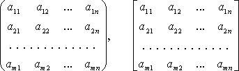
или более кратко
соответственно

Две матрицы А и B
одинаковых размеров равны (запись А
= В), если

— нулевая матрица,

— матрица, противоположная матрице A,

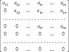
— трапециевидная (ступенчатая) матрица

—
матрица-строка.

—
матрица-столбец,

—
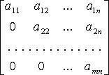верхняя треугольная матрица,

—
нижняя треугольная матрица,

—
диагональная матрица,

—
скалярная матрица,

—
единичная матрица,

(кратко:
где
—
символ Кронекера).

Если все
действительны,
то матрица A называется действительной;
если хотя бы одно из чисел
комплексное,
то матрица называется комплексной.

Сложение матриц

Суммой матриц
и
одинаковых
размеров называется матрица
тех
же размеров, у которой
Обозначение:
C = А + В.

Свойства сложения
матриц: А + В = В + А, (А + В) + С = A + (B +
C), А + 0 = A, А + (-A) = 0,
A,
B, C.

Вычитание матриц

А — В = А + (-В).

Умножение матрицы
на число

Произведением матрицы
на
число
называется
матрица
тех
же размеров, у которой
Обозначение:

Свойства
,
и

Умножение матриц

Произведением матрицы
размером
на
матрицу
размером
назвается
матрица
размером
у
которой
Обозначение:
C = AB.

Свойства AE = EA = A, AO
= OA = O, (AB)D = A(BD),
(AB)
= (A)B
= A(B),
(A + B)D=AD + BD, D(A + B) = DA + DB (при условии,
что указанные операции имеют смысл).

Для квадратных матриц
А и B, вообще говоря,

Транспонирование
матриц

Свойства:

Специальные классы квадратных матриц

Симметрические матрицы:

—
симметрическая

Кососимметрические
матрицы:

—
кососимметрическая

Ортогональные матрицы:

—
ортогональная

Невырожденные
(неособенные) матрицы:

Вырожденные (особенные)
матрицы:

Обратная матрица

Матрица
—
обратная для матрицы A, если

Для квадратной матрицы
A обратная существует тогда и только
тогда, когда

где
—
алгебраические дополнения элементов
матрицы
A.

Свойства:

Элементарные преобразования матрицы

Элементарными
преобразованиями матрицы называют:

1) умножение какой-нибудь
строки (столбца) на отличное от нуля
число;

2) прибавление к
какой-нибудь строке (столбцу) другой ее
строки (столбца), умноженной на произвольное
число;

3) перестановку местами
любых двух строк (столбцов).

Вычисление обратной
матрицы

Если с помощью элементарных
преобразований строк квадратную матрицу
A можно привести к единичной матрице
E, то при таких же элементарных
преобразованиях над матрицей E
получим
.

Пример.

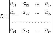
Ранг матрицы

Ранг матрицы — наивысший
порядок отличных от нуля ее миноров.
Обозначение: rank A.

Базисный минор матрицы
— любой отличный от нуля минор порядка
r = rank A.

Системы
линейных уравнений

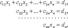
Общий вид системы

,
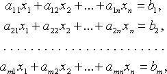
i = 1, 2, …, m; j = 1, 2, …, n, — коэффициенты
системы;
—
свободные члены;
—
переменные;

Если все
=
0, система называется однородной.

Матричная запись
системы линейных уравнений

AX = B,

где

Матрицу A называют
матрицей (или основной матрицей) системы.
Матрицу

называют расширенной матрицей системы,
а матрицу
для
которой AС = В, — вектор-решением
системы.

Критерий совместности
линейных уравнений

Система совместна тогда
и только тогда, когда rank A = rank D.

Правило Крамера

Если m = n и
то
система совместна и имеет единственное
решение
или,
что то же самое,
где
—
определитель, полученный из det A
заменой i-го столбца столбцом
свободных членов.

Общее решение системы линейных
уравнений

Если система линейных
уравнений AX = B совместна, rank A =
r и, например,
—
базисный минор матрицы системы, то она
равносильна системе

Придавая переменным
(свободным
переменным)
получаем
однозначно (например, по правилу Крамера)
Тогда
—
решение исходной системы.

Метод Гаусса

Метод Гаусса — метод
последовательного исключения переменных.
С помощью элементарных преобразований
строк расширенной матрицы D системы
матрицу A системы приводят к
ступенчатому виду:

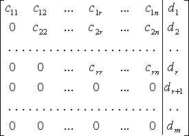
Если
среди чисел
есть
отличные от нуля, система несовместна.

Если
то:

1) при r = n исходная
система равносильна системе:

имеющей единственное решение (сначала
находим из последнего уравнения
,
из предпоследнего
и
т. д.);

2) при r < n исходная система равносильна
системе:

имеющей бесчисленное множество решений
(
— свободные переменные).

Однородные системы
линейных уравнений

Однородная система
линейных уравнений AX = 0 всегда
совместна. Она имеет нетривиальные
(ненулевые) решения, если r = rank A <
n.

Для однородных систем
базисные переменные (коэффициенты при
которых образуют базисный минор)
выражаются через свободные переменные
соотношениями вида:

Тогда n — r линейно
независимыми вектор-решениями будут:

а любое другое решение является их
линейной комбинацией. Вектор-решения
образуют
нормированную фундаментальную систему.

В линейном пространстве
множество
решений однородной системы линейных
уравнений образует подпространство
размерности n — r;
—
базис этого подпространства.

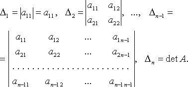
Определители

Определения

В перестановке
чисел
1, 2, …, n два числа
и
составляют
инверсию, если i < j, но
>.
Число всех возможных инверсий данной
перестановки обозначают
Перестановку
называют четной, если I — четное
число, и нечетной, если I — нечетное
число.

Определитель (детерминант)
квадратной матрицы
—
число (обозначение
)

где
означает,
что суммирование производится по всем
перестановкам
чисел
1, 2, …, n.

В частности n = 2

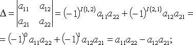
при n = 3

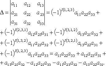
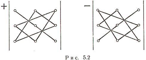
На рис. 5.2 проиллюстрирован
закон, по которому составляется
определитель матрицы третьего порядка:
слева дано правило вычисления положительных
членов определителя, справа — отрицательных.

Миноры определителя

Минор
элемента
определителя
порядка
n — определитель порядка n — 1,
полученный из
вычеркиванием
i-й строки и j-го столбца.

Главные миноры
определителя

Для
главные
миноры есть определители

Алгебраические дополнения

Алгебраическое дополнение
элемента
определителя
—
определитель
где
—
минор элемента
.

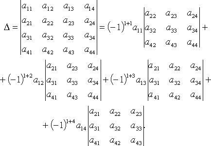
Разложение
определителя

По элементам i-й
строки:

По элементам j-го
столбца:

Например, при n = 4
разложение по первой строке

Свойства определителя

2. Если все элементы
какой-нибудь строки (столбца) определителя
равны нулю, то определитель равен нулю.

3. Если матрица B
получена из матрицы A перестановкой
двух каких-либо ее строе (столбцов), то

4. Общий множитель всех
элементов произвольной строки (столбца)
определителя можно вынести за знак
определителя.

5. Определитель, содержащий
две пропорциональные строки (столбца),
равен нулю.

6. Пусть
—
квадратная матрица порядка n; k
— фиксированное натуральное число:
—
матрицы, которые получаются из A
заменой ее k-й строки (столбца)
соответственно строками (столбцами)
Тогда

7. Определитель не
меняется от прибавления к какой-либо
его строке (столбцу) другой его строки
(столбца), умноженной на произвольное
число.

8. Если какая-либо строка
(столбец) определителя есть линейная
комбинация других его строк (столбцов),
то определитель равен нулю.

Соседние файлы в предмете [НЕСОРТИРОВАННОЕ]

Источник

Краткое содержание прошлых частей:

Линейная алгебра изучает векторы, матрицы и другие понятия, которые относятся к упорядоченным наборам данных. Линейной алгебре интересно, как можно трансформировать эти упорядоченные данные, складывать и умножать, всячески обсчитывать и находить в них закономерности.
Вектор — это набор упорядоченных данных в одном измерении. Можно упрощённо сказать, что это последовательность чисел.
Матрица — это тоже набор упорядоченных данных, только уже не в одном измерении, а в двух (или даже больше).
Матрицу можно представить как упорядоченную сумку с данными. И с этой сумкой как с единым целым можно совершать какие-то действия. Например, делить, умножать, менять знаки.
Матрицы можно складывать и умножать на другие матрицы. Это как взять две сумки с данными и получить третью сумку, тоже с данными, только теперь какими-то новыми.
Матрицы перемножаются по довольно замороченному алгоритму. Арифметика простая, а порядок перемножения довольно запутанный.

И вот наконец мы здесь: если мы можем перемножать матрицы, то мы можем и решить матричное уравнение.

Что такое матричное уравнение

Шаг 1. Упрощаем уравнение

Приводим матричное уравнение к упрощённому виду

Шаг 2. Вводим единичную матрицу

Можно представить, что есть число 100 — это «сто в первой степени», 100¹

И есть число 0,01 — это «сто в минус первой степени», 100^-1

При перемножении этих двух чисел получится единица:
100¹× 100^-1 = 100 × 0,01 = 1.

Вот такое, только в мире матриц.

Зная свойства единичных и обратных матриц, делаем алгебраическое колдунство. Умножаем обе известные матрицы на обратную матрицу А^-1. Неизвестную матрицу Х оставляем без изменений и переписываем уравнение:

А^-1× А × Х = А^-1× В

Добавляем единичную матрицу и упрощаем запись:

А^-1× А = E — единичная матрица

E × Х = А^-1× В — единичная матрица, умноженная на исходную матрицу, даёт исходную матрицу. Единичную матрицу убираем

Х = А^-1× В — новая запись уравнения

💡 Смотрите, что произошло: раньше нам нужно было найти неизвестную матрицу. А теперь мы точно знаем, как её найти: нужно рассчитать обратную матрицу A^-1 и умножить её на известную матрицу B. И то и другое — замороченные процедуры, но с точки зрения арифметики — просто.

Шаг 3. Находим обратную матрицу

Вспоминаем формулу и порядок расчёта обратной матрицы:

Делим единицу на определитель матрицы A.
Считаем транспонированную матрицу алгебраических дополнений.
Перемножаем значения и получаем нужную матрицу.

Формула вычисления обратной матрицы

Первое действие. Мы посчитали определитель и убедились, что он не равен нулю, — это значит, что у матричного уравнения есть вариант решения и можно продолжать

Второе действие, часть 1: получаем матрицу миноров

Второе действие, часть 2: переводим матрицу миноров в транспонированную матрицу алгебраических дополнений

Третье действие: получаем обратную матрицу

Шаг 4. Вычисляем неизвестную матрицу

Нам остаётся посчитать матрицу X: умножаем обратную матрицу А^-1 на матрицу B. Дробь держим за скобками и вносим в матрицу только при условии, что элементы новой матрицы будут кратны десяти — их можно умножить на дробь и получить целое число. Если кратных элементов не будет — дробь оставим за скобками.

Шаг 5. Проверяем уравнение

Проверяем ответ и получаем матрицу B — наши расчёты верны

Ну и что

Этого котика не существует, а матрицы — существуют.

Источник

Метод матричного исчисления

Решение матричных уравнений

Что такое матричное уравнение

Шаг 1. Упрощаем уравнение

Шаг 2. Вводим единичную матрицу

Шаг 3. Находим обратную матрицу

Шаг 4. Вычисляем неизвестную матрицу

Шаг 5. Проверяем уравнение

Ну и что

Онлайн калькулятор. Решение систем линейных уравнений. Матричный метод. Метод обратной матрицы.

Решить систему линейных уравнений матричным методом

Ввод данных в калькулятор для решения систем линейных уравнений матричным методом

Дополнительные возможности калькулятора для решения систем линейных уравнений матричным методом

Решение матричных уравнений: теория и примеры

Решение матричных уравнений: как это делается

Решение матричных уравнений: примеры

Scope[edit]

Relation to other derivatives[edit]

Usages[edit]

Notation[edit]

Alternatives[edit]

Derivatives with vectors[edit]

Vector-by-scalar[edit]

Scalar-by-vector[edit]

Vector-by-vector[edit]

Derivatives with matrices[edit]

Matrix-by-scalar[edit]

Scalar-by-matrix[edit]

Other matrix derivatives[edit]

Layout conventions[edit]

Numerator-layout notation[edit]

Denominator-layout notation[edit]

Identities[edit]

Vector-by-vector identities[edit]

Scalar-by-vector identities[edit]

Vector-by-scalar identities[edit]

Scalar-by-matrix identities[edit]

Matrix-by-scalar identities[edit]

Scalar-by-scalar identities[edit]

With vectors involved[edit]

With matrices involved[edit]

Identities in differential form[edit]

Applications[edit]

See also[edit]

Notes[edit]

References[edit]

Further reading[edit]

External links[edit]

Software[edit]

Information[edit]

Матричное исчисление

Системы линейных уравнений

Определители

Что такое матричное уравнение

Шаг 1. Упрощаем уравнение

Шаг 2. Вводим единичную матрицу

Шаг 3. Находим обратную матрицу

Шаг 4. Вычисляем неизвестную матрицу

Шаг 5. Проверяем уравнение

Ну и что

Не пропустите также:

Матричное
исчисление

Системы
линейных уравнений