Это уравнение вида ax2+bx+c=0ax^2 + bx + c = 0,
где aa – коэффициент перед x2x^2,
bb – коэффициент перед xx,
cc – свободное число.
Существуют разные способы нахождения корней квадратного уравнения. Пожалуй, самый основной и распространенный способ – через вычисление дискриминанта. В этом случае он рассчитывается по формуле:
D=b2–4acD = b^2 – 4ac
Если второй коэффициент уравнения четный, можно решать уравнение через kk, тогда будет другая формула дискриминанта:
D1=k2–acD_1 = k^2 – ac
Если первый коэффициент уравнения равен 1, то можно воспользоваться теоремой Виета, которая имеет 2 условия:
x1+x2=−bx_1 + x_2 = -b
x1⋅x2=cx_1 cdot x_2 = c
Но если мы захотим решить уравнение основным способом, ошибки не будет. Нахождение корней уравнения через дискриминант – универсальный способ, а остальные введены для удобства вычислений.
Задача 1
Решим уравнение: 3×2+7x−6=0.3x^2 + 7x — 6 = 0.
Обозначим коэффициенты:
a=3a = 3,
b=7b = 7,
c=−6c = -6
Далее находим дискриминант по формуле:
D=b2–4acD = b^2 – 4ac
D=72–4∗3∗(−6)=49+72=121=112D = 7^2 – 4 * 3 * (-6) = 49 + 72 = 121 = {11}^2
D>0D > 0 – значит, уравнение имеет 2 корня.
Находим корни уравнения по следующим формулам:
x1=(−b+√D)/2ax_1 = (-b + √D) / 2a
x2=(−b−√D)/2ax_2 = (-b — √D) / 2a
Подставляем численные значения:
x1=(−7+11)/2∗3=4/6=23x_1 = (-7 + 11) / 2*3 = 4 / 6 = frac{2}{3}
x2=(−7–11)/2∗3=−18/6=−3x_2 = (-7 – 11) / 2*3 = -18 / 6 = -3
Ответ: x1=23x_1 = frac{2}{3}, x2=−3x_2 = -3.
Задача 2
Решим уравнение: −x2+7x+8=0.-x^2 + 7x + 8 = 0.
Обозначим коэффициенты:
a=−1a = -1,
b=7b = 7,
c=8.c = 8.
Далее находим дискриминант по формуле:
D=b2–4acD = b^2 – 4ac
D=72–4⋅(−1)⋅8=49+32=81=92D = 7^2 – 4 cdot (-1) cdot 8 = 49 + 32 = 81 = 9^2
D>0D > 0 – значит, уравнение имеет 2 корня.
Находим корни уравнения по следующим формулам:
x1=(−b+√D)/2ax_1 = (-b + √D) / 2a
x2=(−b−√D)/2ax_2 = (-b — √D) / 2a
Подставляем численные значения:
x1=(−7+9)/2∗(−1)=2/(−2)=−1x_1 = (-7 + 9) / 2 * (-1) = 2 / (-2) = -1
x2=(−7–9)/2∗(−1)=−16/(−2)=8x_2 = (-7 – 9) / 2 * (-1) = -16 / (-2) = 8
Ответ: x1=−1x_1 = -1, x2=8x_2 = 8.
Задача 3
Решим уравнение: 4×2+4x+1=0.4x^2 + 4x + 1 = 0.
Обозначим коэффициенты:
a=4a = 4,
b=4b = 4,
c=1.c = 1.
Далее находим дискриминант по формуле: D=b2–4acD = b^2 – 4ac
D=42–4⋅4⋅1=16–16=0D = 4^2 – 4 cdot 4 cdot 1 = 16 – 16 = 0
D=0D = 0 – значит, уравнение имеет 1 корень.
Находим корень уравнения по следующей формуле: x=−b/2ax = -b / 2a
Подставляем численные значения:
x=−4/2⋅4=−4/8=−1/2=−0,5x = -4 / 2 cdot 4 = -4 / 8 = -1 / 2 = -0,5
Ответ: x=−0,5.x = -0,5.
Задача 4
Решим уравнение: 2×2+x+1=0.2x^2 + x + 1 = 0.
Обозначим коэффициенты:
a=2a = 2,
b=1b = 1,
c=1.c = 1.
Далее находим дискриминант по формуле: D=b2–4acD = b^2 – 4ac
D=12–4∗2∗1=1–8=−7D = 1^2 – 4 * 2 * 1 = 1 – 8 = -7
D<0D < 0 – значит, уравнение корней не имеет.
Ответ: корней нет.
Решение квадратного уравнения через k
Если у квадратного уравнения коэффициент bb четный, то можно решать уравнение через kk, при этом k=12bk = frac{1}{2} b.
Задача 5
Решим уравнение: −x2+2x+8=0.-x^2 + 2x + 8 = 0.
Обозначим коэффициенты:
a=−1a = -1,
b=2b = 2,
c=8c = 8
bb – четное.
k=12b=1k = frac {1}{2} b = 1.
Далее находим дискриминант по формуле: D1=k2–acD_1 = k^2 – ac
D1=12–(−1)∗8=1+8=9=32D_1 = 1^2 – (-1) * 8 = 1 + 8 = 9 = 3^2
D1>0D_1 > 0 – значит, уравнение имеет 2 корня.
Находим корни уравнения по следующим формулам:
x1=(−k+D1)/ax_1 = (-k + {sqrt D}_1) / a
x2=(−k−D1)/ax_2 = (-k — {sqrt D}_1) / a
Подставляем численные значения:
x1=(−1+3)/(−1)=2/(−1)=−2x_1 = (-1 + 3) / (-1) = 2 / (-1) = -2
x2=(−1–3)/(−1)=−4/(−1)=4x_2 = (-1 – 3) / (-1) = -4 / (-1) = 4
Ответ: x_1 = -2, x_2 = 4.
Задача 6
Решим уравнение: 9×2–6x+1=0.9x^2 – 6x + 1 = 0.
Обозначим коэффициенты:
a=9a = 9,
b=−6b = -6,
c=1c = 1
bb – четное.
K=12b=−3.K = frac{1}{2} b = -3.
Далее находим дискриминант по формуле: D1=k2–acD_1 = k^2 – ac
D1=(−3)2–9∗1=9–9=0D_1 = {(-3)}^2 – 9 * 1 = 9 – 9 = 0
D1=0D_1 = 0 – значит, уравнение имеет 1 корень.
Находим корень уравнения по следующей формуле: x=−k/ax = -k / a
Подставляем численные значения:
x=3/9=13x = 3 / 9 = frac{1}{3}
Ответ: x=13.x = frac{1}{3}.
Нахождение корней уравнения по теореме Виета
Если в квадратном уравнении a=1a = 1, то можно найти корни уравнения по теореме Виета.
Задача 7
Найдем корни уравнения: x2+3x+2=0.x^2 + 3x + 2 = 0.
Обозначим коэффициенты:
a=1a = 1,
b=3b = 3,
c=2c = 2.
Запишем 2 условия теоремы Виета:
x1+x2=−bx_1 + x_2 = -b
x1∗x2=cx_1 * x_2 = c
Теперь методом подбора найдем 2 числа, которые будут соответствовать этим условиям. Вероятно, это числа -2 и -1.
Значит, корни уравнения равны:
x1=−2x_1 = -2
x2=−1x_2 = -1
Ответ: x1=−2x_1 = -2, x2=−1x_2 = -1.
Задача 8
Найдем корни уравнения: x2–5x+6=0.x^2 – 5x +6 = 0.
Обозначим коэффициенты:
a=1a = 1,
b=−5b = -5,
c=6c = 6
Запишем 2 условия теоремы Виета:
x1+x2=−bx_1 + x_2 = -b
x1∗x2=cx_1 * x_2 = c
Теперь методом подбора найдем 2 числа, которые будут соответствовать этим условиям. Вероятно, это числа 2 и 3.
Значит, корни уравнения равны:
x1=2x_1 = 2
x2=3x_2 = 3
Ответ: x1=2x_1 = 2, x2=3.x_2 = 3.
Тест по теме «Примеры решения квадратных уравнений»
О квадратных уравнениях в правильном порядке
Время на прочтение
4 мин
Количество просмотров 38K
Как вам преподавали квадратные уравнения в школе? Это был 7-8 класс, примерно. Вероятнее всего, вам рассказали что есть формулы корней через дискриминант, что направление ветвей зависит от старшего коэффициента. Через пару занятий дали теорему Виета. Счастливчикам еще рассказали про метод переброски. И на этом решили отпустить.
Вы довольны такой базой? Вам не рассказали ни геометрический смысл, ни как это получить.
Спустя некоторое время обдумывания сей несправедливости, я решил написать эту статью и тем самым закрыть гештальт о фрагментарности знаний.
Вы не найдете здесь ничего нового по факту, но, возможно, это даст посмотреть на такое простое понятие с другой стороны.
Начнем с конца
Когда я перечислял темы, касающиеся квадратных уравнений, я делал это примерно в том же порядке, в котором изучают их в школе. Но такой порядок не оправдан с точки зрения обучения, и вот почему:
-
Дискриминант дается просто как данность (за редким исключением, когда показывают вывод этих формул через приведение к полному квадрату)
-
Мощнейшая по своей сути теорема Виета дается в конце и только как эвристический способ решения
Гораздо проще начать с теоремы Виета.
Рассмотрим квадратный трехчлен
![]()
В силу основной теоремы алгебры (примем её как данность, так как её действительно тяжело доказать), мы знаем, что у этого уравнения должно быть два корня. Допустим, что это некоторые числа  . Тогда можно переписать изначальное уравнение как выражение его корней:
![]()
Оба эти уравнения эквиваленты, так как они оба зануляются в  (первое по определению
  , второе по построению).
Раскрывая скобки, мы получим следующее:
![]()
Откуда приравняв соответствующие коэффициенты с имеющимися, получим знаменитую систему:

Мы только что доказали теорему Виета на случай квадратного трехчлена. Это потрясающий результат: мы начинаем получать некоторую информацию о корнях, которые, как мы предположили, существуют. И этот результат мы будем использовать далее.
Геометрия параболы
Вершина
Здесь можно было бы рассказать весь первый курс алгебры университета: о фокусах, директрисах, о конических сечениях, первой и второй производной…
Но раз мы ограничились школьной программой (7-8 класс, если быть точным), то и рассуждения у нас будут простые.
Самая, на мой субъективный взгляд, интересная точка параболы – это её вершина. Она уникальным образом задает положение параболе и дает понимание о том, как устроены корни.
Но формулу для нее мы не знаем, до первых понятий о производной нам еще 3 года в среднем. Будем выкручиваться.
Парабола – симметричная фигура. До того момента, как мы сдвинули ее относительно оси  , ось
, ось  служит для нее осью симметрии. Когда же мы начинаем ее сдвигать, становится видно, что она продолжает быть симметричной, но уже относительно оси, проходящей через вершину.

Тогда от вершины в обе стороны до корней равные расстояния, а это значит, что вершина параболы лежит ровно между корнями. Тогда координата  вершины это среднее между ее корнями
![]()
Пока что мы не знаем наши корни. Но благодаря теореме Виета мы знаем, чему равна сумма корней!
![]()
Потрясающий результат, который нам пригодится далее.
Ещё немного про корни
Мы знаем, что корни, графически, это те точки, в которых кривая пересекает ось  . Очень полезное знание, учитывая, что смотря на параболу, исключительно визуально, мы понимаем что у нас может быть 3 случая:
-
Корней нет, при этом
-
Либо значение в вершине больше нуля и старший коэффициент больше нуля
-
Либо значение в вершине меньше нуля и старший коэффициент меньше нуля
-
-
Корень один, но кратности 2 (не забываем основную теорему алгебры), и значение в вершине равно нулю
-
Корня два
Второй случай тривиален, до третьего мы еще дойдем. Интересно математически взглянуть на первый. Найдем значение квадратного трехчлена в вершине:

И теперь все же рассмотрим первый случай: парабола висит над осью  ветвями вверх.


Домножим первое неравенство на  . Учитывая, что
  , знак неравенства сменится на противоположный:
![]()
Это условие, при котором корней нет.
Рассмотрим вкратце противоположный случай: парабола висит под осью  ветвями вниз.


![]()
Какая-то магия. Получается, что это условие инвариантно относительно положения параболы. Но тем оно лучше.
На данном этапе прошу заметить, что это только условие отсутствия действительных корней. Да, это похоже на дискриминант, но давайте представим, что вы этого не знаете.
Понятие дискриминанта
Мы уже многое поняли о корнях: в какой они связи с коэффициентами, когда они не существуют, каким образом они лежат относительно вершины. Все это безумно полезно, но это все до сих пор не способ найти значения алгебраически.
Давайте будем отталкиваться от того, что мы уже знаем: от вершины. Если бы мы каким-то образом знали расстояние между корнями, то могли бы однозначно найти и сами корни.
Таки что мешает нам это сделать? Но как настоящие математики, давайте находить квадрат расстояния между корнями. Не теряя общности, будем считать, что  – больший корень. Тогда
![]()
Пока что выглядит не очень, но на что-то это очень сильно похоже. Не видите? Давайте выделим полный квадрат, но по сумме, а не по разности: добавим  , но чтобы все осталось в точности так же, это же и вычтем.
![]()
Все еще не видите? Воспользуемся снова теоремой Виета:
![]()
Мы получили квадрат расстояния между корнями с учетом растяжения коэффициентом  .
.
Так мы теперь можем найти корни! Вершина параболы да половину расстояния между корнями в обе стороны:

Или, немного преобразовав
![]()
Квадрат расстояния между корнями квадратного трехчлена и есть дискриминант.
В общем случае, дискриминант — более сложное понятие, связанное с кратными корнями. Но для квадратного уравнения в 7 классе этого достаточно.
Теперь, если рассуждать о дискриминанте как о расстоянии, становится логично и понятно, почему если он равен нулю, то корень всего один; а если отрицательный, то действительных корней вообще нет.
Заключение
Заметьте, что единственное, что мы предположили, что корня два и они существуют. Единственное, что приняли на веру, это основную теорему алгебры. До всего остального мы дошли исключительно умозрительными заключениями и простейшей алгеброй.
Как по мне, это именно то, как должны преподавать эту тему в школе.
Решение квадратных уравнений
6 июля 2011
Квадратные уравнения изучают в 8 классе, поэтому ничего сложного здесь нет. Умение решать их совершенно необходимо.
Квадратное уравнение — это уравнение вида ax2 + bx + c = 0, где коэффициенты a, b и c — произвольные числа, причем a ≠ 0.
Прежде, чем изучать конкретные методы решения, заметим, что все квадратные уравнения можно условно разделить на три класса:
- Не имеют корней;
- Имеют ровно один корень;
- Имеют два различных корня.
В этом состоит важное отличие квадратных уравнений от линейных, где корень всегда существует и единственен. Как определить, сколько корней имеет уравнение? Для этого существует замечательная вещь — дискриминант.
Дискриминант
Пусть дано квадратное уравнение ax2 + bx + c = 0. Тогда дискриминант — это просто число D = b2 − 4ac.
Эту формулу надо знать наизусть. Откуда она берется — сейчас неважно. Важно другое: по знаку дискриминанта можно определить, сколько корней имеет квадратное уравнение. А именно:
- Если D < 0, корней нет;
- Если D = 0, есть ровно один корень;
- Если D > 0, корней будет два.
Обратите внимание: дискриминант указывает на количество корней, а вовсе не на их знаки, как почему-то многие считают. Взгляните на примеры — и сами все поймете:
Задача. Сколько корней имеют квадратные уравнения:
- x2 − 8x + 12 = 0;
- 5x2 + 3x + 7 = 0;
- x2 − 6x + 9 = 0.
Выпишем коэффициенты для первого уравнения и найдем дискриминант:
a = 1, b = −8, c = 12;
D = (−8)2 − 4 · 1 · 12 = 64 − 48 = 16
Итак, дискриминант положительный, поэтому уравнение имеет два различных корня. Аналогично разбираем второе уравнение:
a = 5; b = 3; c = 7;
D = 32 − 4 · 5 · 7 = 9 − 140 = −131.
Дискриминант отрицательный, корней нет. Осталось последнее уравнение:
a = 1; b = −6; c = 9;
D = (−6)2 − 4 · 1 · 9 = 36 − 36 = 0.
Дискриминант равен нулю — корень будет один.
Обратите внимание, что для каждого уравнения были выписаны коэффициенты. Да, это долго, да, это нудно — зато вы не перепутаете коэффициенты и не допустите глупых ошибок. Выбирайте сами: скорость или качество.
Кстати, если «набить руку», через некоторое время уже не потребуется выписывать все коэффициенты. Такие операции вы будете выполнять в голове. Большинство людей начинают делать так где-то после 50-70 решенных уравнений — в общем, не так и много.
Корни квадратного уравнения
Теперь перейдем, собственно, к решению. Если дискриминант D > 0, корни можно найти по формулам:
![]()
Когда D = 0, можно использовать любую из этих формул — получится одно и то же число, которое и будет ответом. Наконец, если D < 0, корней нет — ничего считать не надо.
Задача. Решить квадратные уравнения:
- x2 − 2x − 3 = 0;
- 15 − 2x − x2 = 0;
- x2 + 12x + 36 = 0.
Первое уравнение:
x2 − 2x − 3 = 0 ⇒ a = 1; b = −2; c = −3;
D = (−2)2 − 4 · 1 · (−3) = 16.
D > 0 ⇒ уравнение имеет два корня. Найдем их:
![]()
Второе уравнение:
15 − 2x − x2 = 0 ⇒ a = −1; b = −2; c = 15;
D = (−2)2 − 4 · (−1) · 15 = 64.
D > 0 ⇒ уравнение снова имеет два корня. Найдем их
[begin{align} & {{x}_{1}}=frac{2+sqrt{64}}{2cdot left( -1 right)}=-5; \ & {{x}_{2}}=frac{2-sqrt{64}}{2cdot left( -1 right)}=3. \ end{align}]
Наконец, третье уравнение:
x2 + 12x + 36 = 0 ⇒ a = 1; b = 12; c = 36;
D = 122 − 4 · 1 · 36 = 0.
D = 0 ⇒ уравнение имеет один корень. Можно использовать любую формулу. Например, первую:
[x=frac{-12+sqrt{0}}{2cdot 1}=-6]
Как видно из примеров, все очень просто. Если знать формулы и уметь считать, проблем не будет. Чаще всего ошибки возникают при подстановке в формулу отрицательных коэффициентов. Здесь опять же поможет прием, описанный выше: смотрите на формулу буквально, расписывайте каждый шаг — и очень скоро избавитесь от ошибок.
Неполные квадратные уравнения
Бывает, что квадратное уравнение несколько отличается от того, что дано в определении. Например:
- x2 + 9x = 0;
- x2 − 16 = 0.
Несложно заметить, что в этих уравнениях отсутствует одно из слагаемых. Такие квадратные уравнения решаются даже легче, чем стандартные: в них даже не потребуется считать дискриминант. Итак, введем новое понятие:
Уравнение ax2 + bx + c = 0 называется неполным квадратным уравнением, если b = 0 или c = 0, т.е. коэффициент при переменной x или свободный элемент равен нулю.
Разумеется, возможен совсем тяжелый случай, когда оба этих коэффициента равны нулю: b = c = 0. В этом случае уравнение принимает вид ax2 = 0. Очевидно, такое уравнение имеет единственный корень: x = 0.
Рассмотрим остальные случаи. Пусть b = 0, тогда получим неполное квадратное уравнение вида ax2 + c = 0. Немного преобразуем его:
![]()
Поскольку арифметический квадратный корень существует только из неотрицательного числа, последнее равенство имеет смысл исключительно при (−c/a) ≥ 0. Вывод:
- Если в неполном квадратном уравнении вида ax2 + c = 0 выполнено неравенство (−c/a) ≥ 0, корней будет два. Формула дана выше;
- Если же (−c/a) < 0, корней нет.
Как видите, дискриминант не потребовался — в неполных квадратных уравнениях вообще нет сложных вычислений. На самом деле даже необязательно помнить неравенство (−c/a) ≥ 0. Достаточно выразить величину x2 и посмотреть, что стоит с другой стороны от знака равенства. Если там положительное число — корней будет два. Если отрицательное — корней не будет вообще.
Теперь разберемся с уравнениями вида ax2 + bx = 0, в которых свободный элемент равен нулю. Тут все просто: корней всегда будет два. Достаточно разложить многочлен на множители:
![]()
Произведение равно нулю, когда хотя бы один из множителей равен нулю. Отсюда находятся корни. В заключение разберем несколько таких уравнений:
Задача. Решить квадратные уравнения:
- x2 − 7x = 0;
- 5x2 + 30 = 0;
- 4x2 − 9 = 0.
x2 − 7x = 0 ⇒ x · (x − 7) = 0 ⇒ x1 = 0; x2 = −(−7)/1 = 7.
5x2 + 30 = 0 ⇒ 5x2 = −30 ⇒ x2 = −6. Корней нет, т.к. квадрат не может быть равен отрицательному числу.
4x2 − 9 = 0 ⇒ 4x2 = 9 ⇒ x2 = 9/4 ⇒ x1 = 3/2 = 1,5; x2 = −1,5.
Смотрите также:
- Теорема Виета

- Следствия из теоремы Виета
- Тест на тему «Значащая часть числа»

- Метод коэффициентов, часть 1
- Однородные тригонометрические уравнения: общая схема решения
- Задача B4: строительные бригады
В предыдущих уроках мы разбирали
«Как решать линейные уравнения», то есть
уравнения первой степени. В этом уроке мы разберем, что называют квадратным уравнением и как его решать.
Что называют квадратным уравнением
Важно!

Степень уравнения определяют по наибольшей степени, в которой
стоит неизвестное.
Если максимальная степень, в которой стоит неизвестное — «2»,
значит, перед вами квадратное уравнение.
Примеры квадратных уравнений
- 5x2 − 14x + 17 = 0
- −x2 + x + = 0
- x2 + 0,25x = 0
- x2 − 8 = 0
Важно!
Общий вид квадратного уравнения выглядит так:
ax2 + bx + c = 0
«a», «b» и «c» — заданные числа.
- «a» — первый или старший коэффициент;
- «b» — второй коэффициент;
- «c» — свободный член.
Чтобы найти «a», «b» и «c»
нужно сравнить свое уравнение с общим видом квадратного уравнения
«ax2 + bx + c = 0».
Давайте потренируемся определять
коэффициенты «a», «b»
и «c» в квадратных уравнениях.
| Уравнение | Коэффициенты | ||||
|---|---|---|---|---|---|
| 5x2 − 14x + 17 = 0 |
|
||||
| −7x2 − 13x + 8 = 0 |
|
||||
−x2 + x +
= 0 |
|
||||
| x2 + 0,25x = 0 |
|
||||
| x2 − 8 = 0 |
|
Как решать квадратные уравнения
В отличии от линейных уравнений для решения квадратных уравнений используется специальная
формула для нахождения корней.
Запомните!
![]()
Чтобы решить квадратное уравнение нужно:
- привести квадратное уравнение к общему виду «ax2 + bx + c = 0».
То есть в правой части должен остаться только «0»; - использовать формулу для корней:
Давайте на примере разберем, как применять формулу для нахождения корней квадратного уравнения. Решим квадратное уравнение.
x2 − 3x − 4 = 0
Уравнение «
x2 − 3x − 4 = 0
» уже приведено к общему виду «ax2 + bx + c = 0» и не требует дополнительных упрощений.
Для его решения нам достаточно применить формулу нахождения корней квадратного уравнения.
Определим коэффициенты «a», «b» и
«c» для этого уравнения.
| Уравнение | Коэффициенты |
|---|---|
| x2 − 3x − 4 = 0 |
|
Подставим их в формулу и найдем корни.
x2 − 3x − 4 = 0
x1;2 =
x1;2 =
| −(−3) ± √(−3)2 − 4 · 1· (−4) |
| 2 · 1 |
x1;2 =
x1;2 =
x1;2 =
| x1 = |
x2 = |
| x1 = |
x2 = |
| x1 = 4 |
x2 = −1 |
Ответ: x1 = 4; x2 = −1
Важно!
Обязательно выучите наизусть формулу для нахождения корней.
С её помощью решается любое квадратное уравнение.
В формуле «x1;2 = » часто заменяют подкоренное выражение
«b2 − 4ac» на букву «D» и называют
дискриминантом. Более подробно понятие дискриминанта рассматривается в уроке
«Что такое дискриминант».
Рассмотрим другой пример квадратного уравнения.
x2 + 9 + x = 7x
В данном виде определить коэффициенты «a», «b» и
«c» довольно сложно.
Давайте вначале приведем уравнение к общему виду «ax2 + bx + c = 0».
Используем
правило переноса и
упростим подобные
члены.
x2 + 9 + x = 7x
x2 + 9 + x − 7x = 0
x2 + 9 − 6x = 0
x2 − 6x + 9 = 0
Теперь можно использовать формулу для корней.
x1;2 =
| −(−6) ± √(−6)2 − 4 · 1 · 9 |
| 2 · 1 |
x1;2 =
x1;2 =
x1;2 =
x =
x = 3
Ответ: x = 3
Бывают случаи, когда в квадратных уравнениях нет корней. Такая ситуация возникает, когда в формуле под корнем
оказывается отрицательное число.
Мы помним из определения квадратного корня о том,
что извлекать квадратный корень из отрицательного числа
нельзя.
Рассмотрим пример квадратного уравнения, у которого нет корней.
5x2 + 2x = − 3
5x2 + 2x + 3 = 0
x1;2 =
| −2 ± √22 − 4 · 3 · 5 |
| 2 · 5 |
x1;2 =
x1;2 =
Ответ: нет действительных корней.
Итак, мы получили ситуацию, когда под корнем стоит отрицательное число.
Это означает, что в уравнении нет корней. Поэтому в ответ мы так и записали «Нет действительных корней».
Важно!
Что означают слова «нет действительных корней»? Почему нельзя просто написать «нет корней»?
На самом деле корни в таких случаях есть, но в рамках школьной программы они не проходятся, поэтому и в
ответ мы записываем, что среди действительных чисел корней нет. Другими словами «Нет действительных корней».
Неполные квадратные уравнения
Иногда встречаются квадратные уравнения, в которых отсутсвуют в явном виде коэффициенты «b» и/или
«c». Как например, в таком уравнении:
4x2 − 64 = 0
Такие уравнения называют неполными квадратными уравнениями. Как их решать рассмотрено в уроке
«Неполные квадратные уравнения».
Ваши комментарии
Важно!
Чтобы оставить комментарий, вам нужно войти на наш сайт при помощи
«ВКонтакте».

Оставить комментарий:
8 мая 2018 в 19:54
Safie Bekirova

Профиль
Благодарили: 0
Сообщений: 1
Safie Bekirova
Профиль
Благодарили: 0
Сообщений: 1
0,5х(4х2-1)(5х2+2)
0
Спасибо
Ответить
10 мая 2018 в 10:09
Ответ для Safie Bekirova
Ульяночка Звонкова

Профиль
Благодарили: 0
Сообщений: 1
Ульяночка Звонкова
Профиль
Благодарили: 0
Сообщений: 1
вродебы-2,5
0
Спасибо
Ответить
29 ноября 2015 в 15:30
Евгения Краснова

Профиль
Благодарили: 0
Сообщений: 1
Евгения Краснова
Профиль
Благодарили: 0
Сообщений: 1
Не можем решить уравнение: (х+1)2015 + (х+1)2014 * (х-1) + (х+1)2013 * (х-1)2 +…..+ (х-1)2015 = 0 2015,2014,2013 и 2 — это степени
0
Спасибо
Ответить
12 июня 2016 в 1:55
Ответ для Евгения Краснова
Евгений Фёдоров

Профиль
Благодарили: 0
Сообщений: 60
Евгений Фёдоров
Профиль
Благодарили: 0
Сообщений: 60
Ответ: x = 0.
y = .
1 + y + y2 +… + y2015 = = 0.
0
Спасибо
Ответить
12 августа 2015 в 23:35
Наталья Афонина

Профиль
Благодарили: 0
Сообщений: 1
Наталья Афонина
Профиль
Благодарили: 0
Сообщений: 1
(x2-4)|x|+3=0
0
Спасибо
Ответить
9 июня 2016 в 14:40
Ответ для Наталья Афонина
Евгений Фёдоров
Профиль
Благодарили: 0
Сообщений: 60
Евгений Фёдоров
Профиль
Благодарили: 0
Сообщений: 60
±1; ±(?13 ? 1)/2.
0
Спасибо
Ответить
9 августа 2015 в 20:06
Andrey Porshnev

Профиль
Благодарили: 0
Сообщений: 2
Andrey Porshnev
Профиль
Благодарили: 0
Сообщений: 2
x2-3x-4 Как преобразовать это выражение к виду (x-4)?
Подскажите пожалуйста)
0
Спасибо
Ответить
20 августа 2015 в 11:34
Ответ для Andrey Porshnev
Борис Гуров

Профиль
Благодарили: 1
Сообщений: 28
Борис Гуров
Профиль
Благодарили: 1
Сообщений: 28
Здравствуй, Андрей.
Сперва тебе необходимо найти корни своего уравнения по формуле:
x1;2 =
После этого достаточно воспользоваться формулой:
ax2 + bx + c = a (x — x1)(x — x2), где x1 и x2 — корни уравнения.
0
Спасибо
Ответить
This article is about algebraic equations of degree two and their solutions. For the formula used to find solutions to such equations, see Quadratic formula. For functions defined by polynomials of degree two, see Quadratic function.
In algebra, a quadratic equation (from Latin quadratus ‘square’) is any equation that can be rearranged in standard form as[1]

where x represents an unknown value, and a, b, and c represent known numbers, where a ≠ 0. (If a = 0 and b ≠ 0 then the equation is linear, not quadratic.) The numbers a, b, and c are the coefficients of the equation and may be distinguished by respectively calling them, the quadratic coefficient, the linear coefficient and the constant coefficient or free term.[2]
The values of x that satisfy the equation are called solutions of the equation, and roots or zeros of the expression on its left-hand side. A quadratic equation has at most two solutions. If there is only one solution, one says that it is a double root. If all the coefficients are real numbers, there are either two real solutions, or a single real double root, or two complex solutions that are complex conjugates of each other. A quadratic equation always has two roots, if complex roots are included; and a double root is counted for two. A quadratic equation can be factored into an equivalent equation[3]

where r and s are the solutions for x.
The quadratic formula

expresses the solutions in terms of a, b, and c. Completing the square is one of several ways for deriving the formula.
Solutions to problems that can be expressed in terms of quadratic equations were known as early as 2000 BC.[4][5]
Because the quadratic equation involves only one unknown, it is called «univariate». The quadratic equation contains only powers of x that are non-negative integers, and therefore it is a polynomial equation. In particular, it is a second-degree polynomial equation, since the greatest power is two.
Solving the quadratic equation[edit]

Figure 1. Plots of quadratic function y = ax2 + bx + c, varying each coefficient separately while the other coefficients are fixed (at values a = 1, b = 0, c = 0)
A quadratic equation with real or complex coefficients has two solutions, called roots. These two solutions may or may not be distinct, and they may or may not be real.
Factoring by inspection[edit]
It may be possible to express a quadratic equation ax2 + bx + c = 0 as a product (px + q)(rx + s) = 0. In some cases, it is possible, by simple inspection, to determine values of p, q, r, and s that make the two forms equivalent to one another. If the quadratic equation is written in the second form, then the «Zero Factor Property» states that the quadratic equation is satisfied if px + q = 0 or rx + s = 0. Solving these two linear equations provides the roots of the quadratic.
For most students, factoring by inspection is the first method of solving quadratic equations to which they are exposed.[6]: 202–207 If one is given a quadratic equation in the form x2 + bx + c = 0, the sought factorization has the form (x + q)(x + s), and one has to find two numbers q and s that add up to b and whose product is c (this is sometimes called «Vieta’s rule»[7] and is related to Vieta’s formulas). As an example, x2 + 5x + 6 factors as (x + 3)(x + 2). The more general case where a does not equal 1 can require a considerable effort in trial and error guess-and-check, assuming that it can be factored at all by inspection.
Except for special cases such as where b = 0 or c = 0, factoring by inspection only works for quadratic equations that have rational roots. This means that the great majority of quadratic equations that arise in practical applications cannot be solved by factoring by inspection.[6]: 207
Completing the square[edit]
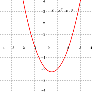
Figure 2. For the quadratic function y = x2 − x − 2, the points where the graph crosses the x-axis, x = −1 and x = 2, are the solutions of the quadratic equation x2 − x − 2 = 0.
The process of completing the square makes use of the algebraic identity

which represents a well-defined algorithm that can be used to solve any quadratic equation.[6]: 207 Starting with a quadratic equation in standard form, ax2 + bx + c = 0
- Divide each side by a, the coefficient of the squared term.
- Subtract the constant term c/a from both sides.
- Add the square of one-half of b/a, the coefficient of x, to both sides. This «completes the square», converting the left side into a perfect square.
- Write the left side as a square and simplify the right side if necessary.
- Produce two linear equations by equating the square root of the left side with the positive and negative square roots of the right side.
- Solve each of the two linear equations.
We illustrate use of this algorithm by solving 2x2 + 4x − 4 = 0


The plus–minus symbol «±» indicates that both x = −1 + √3 and x = −1 − √3 are solutions of the quadratic equation.[8]
Quadratic formula and its derivation[edit]
Completing the square can be used to derive a general formula for solving quadratic equations, called the quadratic formula.[9] The mathematical proof will now be briefly summarized.[10] It can easily be seen, by polynomial expansion, that the following equation is equivalent to the quadratic equation:

Taking the square root of both sides, and isolating x, gives:

Some sources, particularly older ones, use alternative parameterizations of the quadratic equation such as ax2 + 2bx + c = 0 or ax2 − 2bx + c = 0 ,[11] where b has a magnitude one half of the more common one, possibly with opposite sign. These result in slightly different forms for the solution, but are otherwise equivalent.
A number of alternative derivations can be found in the literature. These proofs are simpler than the standard completing the square method, represent interesting applications of other frequently used techniques in algebra, or offer insight into other areas of mathematics.
A lesser known quadratic formula, as used in Muller’s method, provides the same roots via the equation

This can be deduced from the standard quadratic formula by Vieta’s formulas, which assert that the product of the roots is c/a. It also follows from dividing the quadratic equation by  giving
  solving this for
  and then inverting.
One property of this form is that it yields one valid root when a = 0, while the other root contains division by zero, because when a = 0, the quadratic equation becomes a linear equation, which has one root. By contrast, in this case, the more common formula has a division by zero for one root and an indeterminate form 0/0 for the other root. On the other hand, when c = 0, the more common formula yields two correct roots whereas this form yields the zero root and an indeterminate form 0/0.
When neither a nor c is zero, the equality between the standard quadratic formula and Muller’s method,

can be verified by cross multiplication, and similarly for the other choice of signs.
Reduced quadratic equation[edit]
It is sometimes convenient to reduce a quadratic equation so that its leading coefficient is one. This is done by dividing both sides by a, which is always possible since a is non-zero. This produces the reduced quadratic equation:[12]

where p = b/a and q = c/a. This monic polynomial equation has the same solutions as the original.
The quadratic formula for the solutions of the reduced quadratic equation, written in terms of its coefficients, is:

or equivalently:

Discriminant[edit]

Figure 3. Discriminant signs
In the quadratic formula, the expression underneath the square root sign is called the discriminant of the quadratic equation, and is often represented using an upper case D or an upper case Greek delta:[13]

A quadratic equation with real coefficients can have either one or two distinct real roots, or two distinct complex roots. In this case the discriminant determines the number and nature of the roots. There are three cases:
- If the discriminant is positive, then there are two distinct roots
-
- both of which are real numbers. For quadratic equations with rational coefficients, if the discriminant is a square number, then the roots are rational—in other cases they may be quadratic irrationals.

- If the discriminant is zero, then there is exactly one real root
 sometimes called a repeated or double root.

- If the discriminant is negative, then there are no real roots. Rather, there are two distinct (non-real) complex roots[14]

- which are complex conjugates of each other. In these expressions i is the imaginary unit.
Thus the roots are distinct if and only if the discriminant is non-zero, and the roots are real if and only if the discriminant is non-negative.
Geometric interpretation[edit]

Graph of y = ax2 + bx + c, where a and the discriminant b2 − 4ac are positive, with
- Roots and y-intercept in red
- Vertex and axis of symmetry in blue
- Focus and directrix in pink

Visualisation of the complex roots of y = ax2 + bx + c: the parabola is rotated 180° about its vertex (orange). Its x-intercepts are rotated 90° around their mid-point, and the Cartesian plane is interpreted as the complex plane (green).[15]
The function f(x) = ax2 + bx + c is a quadratic function.[16] The graph of any quadratic function has the same general shape, which is called a parabola. The location and size of the parabola, and how it opens, depend on the values of a, b, and c. As shown in Figure 1, if a > 0, the parabola has a minimum point and opens upward. If a < 0, the parabola has a maximum point and opens downward. The extreme point of the parabola, whether minimum or maximum, corresponds to its vertex. The x-coordinate of the vertex will be located at  , and the y-coordinate of the vertex may be found by substituting this x-value into the function. The y-intercept is located at the point (0, c).
The solutions of the quadratic equation ax2 + bx + c = 0 correspond to the roots of the function f(x) = ax2 + bx + c, since they are the values of x for which f(x) = 0. As shown in Figure 2, if a, b, and c are real numbers and the domain of f is the set of real numbers, then the roots of f are exactly the x-coordinates of the points where the graph touches the x-axis. As shown in Figure 3, if the discriminant is positive, the graph touches the x-axis at two points; if zero, the graph touches at one point; and if negative, the graph does not touch the x-axis.
Quadratic factorization[edit]
The term

is a factor of the polynomial

if and only if r is a root of the quadratic equation

It follows from the quadratic formula that

In the special case b2 = 4ac where the quadratic has only one distinct root (i.e. the discriminant is zero), the quadratic polynomial can be factored as

Graphical solution[edit]
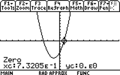
Figure 4. Graphing calculator computation of one of the two roots of the quadratic equation 2x2 + 4x − 4 = 0. Although the display shows only five significant figures of accuracy, the retrieved value of xc is 0.732050807569, accurate to twelve significant figures.

A quadratic function without real root: y = (x − 5)2 + 9. The «3» is the imaginary part of the x-intercept. The real part is the x-coordinate of the vertex. Thus the roots are 5 ± 3i.
The solutions of the quadratic equation
may be deduced from the graph of the quadratic function

which is a parabola.
If the parabola intersects the x-axis in two points, there are two real roots, which are the x-coordinates of these two points (also called x-intercept).
If the parabola is tangent to the x-axis, there is a double root, which is the x-coordinate of the contact point between the graph and parabola.
If the parabola does not intersect the x-axis, there are two complex conjugate roots. Although these roots cannot be visualized on the graph, their real and imaginary parts can be.[17]
Let h and k be respectively the x-coordinate and the y-coordinate of the vertex of the parabola (that is the point with maximal or minimal y-coordinate. The quadratic function may be rewritten

Let d be the distance between the point of y-coordinate 2k on the axis of the parabola, and a point on the parabola with the same y-coordinate (see the figure; there are two such points, which give the same distance, because of the symmetry of the parabola). Then the real part of the roots is h, and their imaginary part are ±d. That is, the roots are

or in the case of the example of the figure

Avoiding loss of significance[edit]
Although the quadratic formula provides an exact solution, the result is not exact if real numbers are approximated during the computation, as usual in numerical analysis, where real numbers are approximated by floating point numbers (called «reals» in many programming languages). In this context, the quadratic formula is not completely stable.
This occurs when the roots have different order of magnitude, or, equivalently, when b2 and b2 − 4ac are close in magnitude. In this case, the subtraction of two nearly equal numbers will cause loss of significance or catastrophic cancellation in the smaller root. To avoid this, the root that is smaller in magnitude, r, can be computed as  where R is the root that is bigger in magnitude. This is equivalent to using the formula

using the plus sign if  and the minus sign if
A second form of cancellation can occur between the terms b2 and 4ac of the discriminant, that is when the two roots are very close. This can lead to loss of up to half of correct significant figures in the roots.[11][18]
Examples and applications[edit]

The golden ratio is found as the positive solution of the quadratic equation 
The equations of the circle and the other conic sections—ellipses, parabolas, and hyperbolas—are quadratic equations in two variables.
Given the cosine or sine of an angle, finding the cosine or sine of the angle that is half as large involves solving a quadratic equation.
The process of simplifying expressions involving the square root of an expression involving the square root of another expression involves finding the two solutions of a quadratic equation.
Descartes’ theorem states that for every four kissing (mutually tangent) circles, their radii satisfy a particular quadratic equation.
The equation given by Fuss’ theorem, giving the relation among the radius of a bicentric quadrilateral’s inscribed circle, the radius of its circumscribed circle, and the distance between the centers of those circles, can be expressed as a quadratic equation for which the distance between the two circles’ centers in terms of their radii is one of the solutions. The other solution of the same equation in terms of the relevant radii gives the distance between the circumscribed circle’s center and the center of the excircle of an ex-tangential quadrilateral.
Critical points of a cubic function and inflection points of a quartic function are found by solving a quadratic equation.
History[edit]
Babylonian mathematicians, as early as 2000 BC (displayed on Old Babylonian clay tablets) could solve problems relating the areas and sides of rectangles. There is evidence dating this algorithm as far back as the Third Dynasty of Ur.[19] In modern notation, the problems typically involved solving a pair of simultaneous equations of the form:

which is equivalent to the statement that x and y are the roots of the equation:[20]: 86

The steps given by Babylonian scribes for solving the above rectangle problem, in terms of x and y, were as follows:
- Compute half of p.
- Square the result.
- Subtract q.
- Find the (positive) square root using a table of squares.
- Add together the results of steps (1) and (4) to give x.
In modern notation this means calculating  , which is equivalent to the modern day quadratic formula for the larger real root (if any)
  with a = 1, b = −p, and c = q.
Geometric methods were used to solve quadratic equations in Babylonia, Egypt, Greece, China, and India. The Egyptian Berlin Papyrus, dating back to the Middle Kingdom (2050 BC to 1650 BC), contains the solution to a two-term quadratic equation.[21] Babylonian mathematicians from circa 400 BC and Chinese mathematicians from circa 200 BC used geometric methods of dissection to solve quadratic equations with positive roots.[22][23] Rules for quadratic equations were given in The Nine Chapters on the Mathematical Art, a Chinese treatise on mathematics.[23][24] These early geometric methods do not appear to have had a general formula. Euclid, the Greek mathematician, produced a more abstract geometrical method around 300 BC. With a purely geometric approach Pythagoras and Euclid created a general procedure to find solutions of the quadratic equation. In his work Arithmetica, the Greek mathematician Diophantus solved the quadratic equation, but giving only one root, even when both roots were positive.[25]
In 628 AD, Brahmagupta, an Indian mathematician, gave the first explicit (although still not completely general) solution of the quadratic equation ax2 + bx = c as follows: «To the absolute number multiplied by four times the [coefficient of the] square, add the square of the [coefficient of the] middle term; the square root of the same, less the [coefficient of the] middle term, being divided by twice the [coefficient of the] square is the value.» (Brahmasphutasiddhanta, Colebrook translation, 1817, page 346)[20]: 87 This is equivalent to

The Bakhshali Manuscript written in India in the 7th century AD contained an algebraic formula for solving quadratic equations, as well as quadratic indeterminate equations (originally of type ax/c = y[clarification needed : this is linear, not quadratic]). Muhammad ibn Musa al-Khwarizmi (9th century), possibly inspired by Brahmagupta,[original research?] developed a set of formulas that worked for positive solutions. Al-Khwarizmi goes further in providing a full solution to the general quadratic equation, accepting one or two numerical answers for every quadratic equation, while providing geometric proofs in the process.[26] He also described the method of completing the square and recognized that the discriminant must be positive,[26][27]: 230 which was proven by his contemporary ‘Abd al-Hamīd ibn Turk (Central Asia, 9th century) who gave geometric figures to prove that if the discriminant is negative, a quadratic equation has no solution.[27]: 234 While al-Khwarizmi himself did not accept negative solutions, later Islamic mathematicians that succeeded him accepted negative solutions,[26]: 191 as well as irrational numbers as solutions.[28] Abū Kāmil Shujā ibn Aslam (Egypt, 10th century) in particular was the first to accept irrational numbers (often in the form of a square root, cube root or fourth root) as solutions to quadratic equations or as coefficients in an equation.[29] The 9th century Indian mathematician Sridhara wrote down rules for solving quadratic equations.[30]
The Jewish mathematician Abraham bar Hiyya Ha-Nasi (12th century, Spain) authored the first European book to include the full solution to the general quadratic equation.[31] His solution was largely based on Al-Khwarizmi’s work.[26] The writing of the Chinese mathematician Yang Hui (1238–1298 AD) is the first known one in which quadratic equations with negative coefficients of ‘x’ appear, although he attributes this to the earlier Liu Yi.[32] By 1545 Gerolamo Cardano compiled the works related to the quadratic equations. The quadratic formula covering all cases was first obtained by Simon Stevin in 1594.[33] In 1637 René Descartes published La Géométrie containing the quadratic formula in the form we know today.
Advanced topics[edit]
Alternative methods of root calculation[edit]
Vieta’s formulas[edit]

Graph of the difference between Vieta’s approximation for the smallest root of the quadratic equation x2 + bx + c = 0 compared with the value calculated using the quadratic formula
Vieta’s formulas (named after François Viète) are the relations

between the roots of a quadratic polynomial and its coefficients. They result from comparing term by term the relation

with the equation

The first Vieta’s formula is useful for graphing a quadratic function. Since the graph is symmetric with respect to a vertical line through the vertex, the vertex’s x-coordinate is located at the average of the roots (or intercepts). Thus the x-coordinate of the vertex is

The y-coordinate can be obtained by substituting the above result into the given quadratic equation, giving

These formulas for the vertex can also deduced directly from the formula (see Completing the square)

For numerical computation, Vieta’s formulas provide a useful method for finding the roots of a quadratic equation in the case where one root is much smaller than the other. If |x2| << |x1|, then x1 + x2 ≈ x1, and we have the estimate:

The second Vieta’s formula then provides:

These formulas are much easier to evaluate than the quadratic formula under the condition of one large and one small root, because the quadratic formula evaluates the small root as the difference of two very nearly equal numbers (the case of large b), which causes round-off error in a numerical evaluation. The figure shows the difference between[clarification needed] (i) a direct evaluation using the quadratic formula (accurate when the roots are near each other in value) and (ii) an evaluation based upon the above approximation of Vieta’s formulas (accurate when the roots are widely spaced). As the linear coefficient b increases, initially the quadratic formula is accurate, and the approximate formula improves in accuracy, leading to a smaller difference between the methods as b increases. However, at some point the quadratic formula begins to lose accuracy because of round off error, while the approximate method continues to improve. Consequently, the difference between the methods begins to increase as the quadratic formula becomes worse and worse.
This situation arises commonly in amplifier design, where widely separated roots are desired to ensure a stable operation (see Step response).
Trigonometric solution[edit]
In the days before calculators, people would use mathematical tables—lists of numbers showing the results of calculation with varying arguments—to simplify and speed up computation. Tables of logarithms and trigonometric functions were common in math and science textbooks. Specialized tables were published for applications such as astronomy, celestial navigation and statistics. Methods of numerical approximation existed, called prosthaphaeresis, that offered shortcuts around time-consuming operations such as multiplication and taking powers and roots.[34] Astronomers, especially, were concerned with methods that could speed up the long series of computations involved in celestial mechanics calculations.
It is within this context that we may understand the development of means of solving quadratic equations by the aid of trigonometric substitution. Consider the following alternate form of the quadratic equation,
[1] 
where the sign of the ± symbol is chosen so that a and c may both be positive. By substituting
[2] 
and then multiplying through by cos2(θ) / c, we obtain
[3] 
Introducing functions of 2θ and rearranging, we obtain
[4] 
[5] 
where the subscripts n and p correspond, respectively, to the use of a negative or positive sign in equation [1]. Substituting the two values of θn or θp found from equations [4] or [5] into [2] gives the required roots of [1]. Complex roots occur in the solution based on equation [5] if the absolute value of sin 2θp exceeds unity. The amount of effort involved in solving quadratic equations using this mixed trigonometric and logarithmic table look-up strategy was two-thirds the effort using logarithmic tables alone.[35] Calculating complex roots would require using a different trigonometric form.[36]
- To illustrate, let us assume we had available seven-place logarithm and trigonometric tables, and wished to solve the following to six-significant-figure accuracy:
-

- A seven-place lookup table might have only 100,000 entries, and computing intermediate results to seven places would generally require interpolation between adjacent entries.
- (rounded to six significant figures)


Solution for complex roots in polar coordinates[edit]
If the quadratic equation  with real coefficients has two complex roots—the case where
  requiring a and c to have the same sign as each other—then the solutions for the roots can be expressed in polar form as[37]

where  and
and 
Geometric solution[edit]
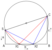
Figure 6. Geometric solution of ax2 + bx + c = 0 using Lill’s method. Solutions are −AX1/SA, −AX2/SA
The quadratic equation may be solved geometrically in a number of ways. One way is via Lill’s method. The three coefficients a, b, c are drawn with right angles between them as in SA, AB, and BC in Figure 6. A circle is drawn with the start and end point SC as a diameter. If this cuts the middle line AB of the three then the equation has a solution, and the solutions are given by negative of the distance along this line from A divided by the first coefficient a or SA. If a is 1 the coefficients may be read off directly. Thus the solutions in the diagram are −AX1/SA and −AX2/SA.[38]

Carlyle circle of the quadratic equation x2 − sx + p = 0.
The Carlyle circle, named after Thomas Carlyle, has the property that the solutions of the quadratic equation are the horizontal coordinates of the intersections of the circle with the horizontal axis.[39] Carlyle circles have been used to develop ruler-and-compass constructions of regular polygons.
Generalization of quadratic equation[edit]
The formula and its derivation remain correct if the coefficients a, b and c are complex numbers, or more generally members of any field whose characteristic is not 2. (In a field of characteristic 2, the element 2a is zero and it is impossible to divide by it.)
The symbol

in the formula should be understood as «either of the two elements whose square is b2 − 4ac, if such elements exist». In some fields, some elements have no square roots and some have two; only zero has just one square root, except in fields of characteristic 2. Even if a field does not contain a square root of some number, there is always a quadratic extension field which does, so the quadratic formula will always make sense as a formula in that extension field.
Characteristic 2[edit]
In a field of characteristic 2, the quadratic formula, which relies on 2 being a unit, does not hold. Consider the monic quadratic polynomial

over a field of characteristic 2. If b = 0, then the solution reduces to extracting a square root, so the solution is

and there is only one root since

In summary,

See quadratic residue for more information about extracting square roots in finite fields.
In the case that b ≠ 0, there are two distinct roots, but if the polynomial is irreducible, they cannot be expressed in terms of square roots of numbers in the coefficient field. Instead, define the 2-root R(c) of c to be a root of the polynomial x2 + x + c, an element of the splitting field of that polynomial. One verifies that R(c) + 1 is also a root. In terms of the 2-root operation, the two roots of the (non-monic) quadratic ax2 + bx + c are

and

For example, let a denote a multiplicative generator of the group of units of F4, the Galois field of order four (thus a and a + 1 are roots of x2 + x + 1 over F4. Because (a + 1)2 = a, a + 1 is the unique solution of the quadratic equation x2 + a = 0. On the other hand, the polynomial x2 + ax + 1 is irreducible over F4, but it splits over F16, where it has the two roots ab and ab + a, where b is a root of x2 + x + a in F16.
This is a special case of Artin–Schreier theory.
See also[edit]
- Solving quadratic equations with continued fractions
- Linear equation
- Cubic function
- Quartic equation
- Quintic equation
- Fundamental theorem of algebra
References[edit]
- ^ Charles P. McKeague (2014). Intermediate Algebra with Trigonometry (reprinted ed.). Academic Press. p. 219. ISBN 978-1-4832-1875-5. Extract of page 219
- ^ Protters & Morrey: «Calculus and Analytic Geometry. First Course».
- ^ The Princeton Review (2020). Princeton Review SAT Prep, 2021: 5 Practice Tests + Review & Techniques + Online Tools. Random House Children’s Books. p. 360. ISBN 978-0-525-56974-9. Extract of page 360
- ^ David Mumford; Caroline Series; David Wright (2002). Indra’s Pearls: The Vision of Felix Klein (illustrated, reprinted ed.). Cambridge University Press. p. 37. ISBN 978-0-521-35253-6. Extract of page 37
- ^ Mathematics in Action Teachers’ Resource Book 4b (illustrated ed.). Nelson Thornes. 1996. p. 26. ISBN 978-0-17-431439-4. Extract of page 26
- ^ a b c Washington, Allyn J. (2000). Basic Technical Mathematics with Calculus, Seventh Edition. Addison Wesley Longman, Inc. ISBN 978-0-201-35666-3.
- ^ Ebbinghaus, Heinz-Dieter; Ewing, John H. (1991), Numbers, Graduate Texts in Mathematics, vol. 123, Springer, p. 77, ISBN 9780387974972.
- ^ Sterling, Mary Jane (2010), Algebra I For Dummies, Wiley Publishing, p. 219, ISBN 978-0-470-55964-2
- ^ Rich, Barnett; Schmidt, Philip (2004), Schaum’s Outline of Theory and Problems of Elementary Algebra, The McGraw-Hill Companies, ISBN 978-0-07-141083-0, Chapter 13 §4.4, p. 291
- ^ Himonas, Alex. Calculus for Business and Social Sciences, p. 64 (Richard Dennis Publications, 2001).
- ^ a b Kahan, Willian (November 20, 2004), On the Cost of Floating-Point Computation Without Extra-Precise Arithmetic (PDF), retrieved 2012-12-25
- ^ Alenit͡syn, Aleksandr and Butikov, Evgeniĭ. Concise Handbook of Mathematics and Physics, p. 38 (CRC Press 1997)
- ^ Δ is the initial of the Greek word Διακρίνουσα, Diakrínousa, discriminant.
- ^ Achatz, Thomas; Anderson, John G.; McKenzie, Kathleen (2005). Technical Shop Mathematics. Industrial Press. p. 277. ISBN 978-0-8311-3086-2.
- ^ «Complex Roots Made Visible – Math Fun Facts». Retrieved 1 October 2016.
- ^ Wharton, P. (2006). Essentials of Edexcel Gcse Math/Higher. Lonsdale. p. 63. ISBN 978-1-905-129-78-2.
- ^ Alec Norton, Benjamin Lotto (June 1984), «Complex Roots Made Visible», The College Mathematics Journal, 15 (3): 248–249, doi:10.2307/2686333, JSTOR 2686333
- ^ Higham, Nicholas (2002), Accuracy and Stability of Numerical Algorithms (2nd ed.), SIAM, p. 10, ISBN 978-0-89871-521-7
- ^ Friberg, Jöran (2009). «A Geometric Algorithm with Solutions to Quadratic Equations in a Sumerian Juridical Document from Ur III Umma». Cuneiform Digital Library Journal. 3.
- ^ a b Stillwell, John (2004). Mathematics and Its History (2nd ed.). Springer. ISBN 978-0-387-95336-6.
- ^ The Cambridge Ancient History Part 2 Early History of the Middle East. Cambridge University Press. 1971. p. 530. ISBN 978-0-521-07791-0.
- ^ Henderson, David W. «Geometric Solutions of Quadratic and Cubic Equations». Mathematics Department, Cornell University. Retrieved 28 April 2013.
- ^ a b Aitken, Wayne. «A Chinese Classic: The Nine Chapters» (PDF). Mathematics Department, California State University. Retrieved 28 April 2013.
- ^ Smith, David Eugene (1958). History of Mathematics. Courier Dover Publications. p. 380. ISBN 978-0-486-20430-7.
- ^ Smith, David Eugene (1958). History of Mathematics, Volume 1. Courier Dover Publications. p. 134. ISBN 978-0-486-20429-1. Extract of page 134
- ^ a b c d Katz, V. J.; Barton, B. (2006). «Stages in the History of Algebra with Implications for Teaching». Educational Studies in Mathematics. 66 (2): 185–201. doi:10.1007/s10649-006-9023-7. S2CID 120363574.
- ^ a b Boyer, Carl B.; Uta C. Merzbach, rev. editor (1991). A History of Mathematics. John Wiley & Sons, Inc. ISBN 978-0-471-54397-8.
- ^ O’Connor, John J.; Robertson, Edmund F. (1999), «Arabic mathematics: forgotten brilliance?», MacTutor History of Mathematics archive, University of St Andrews «Algebra was a unifying theory which allowed rational numbers, irrational numbers, geometrical magnitudes, etc., to all be treated as «algebraic objects».»
- ^ Jacques Sesiano, «Islamic mathematics», p. 148, in Selin, Helaine; D’Ambrosio, Ubiratan, eds. (2000), Mathematics Across Cultures: The History of Non-Western Mathematics, Springer, ISBN 978-1-4020-0260-1
- ^ Smith, David Eugene (1958). History of Mathematics. Courier Dover Publications. p. 280. ISBN 978-0-486-20429-1.
- ^ Livio, Mario (2006). The Equation that Couldn’t Be Solved. Simon & Schuster. ISBN 978-0743258210.
- ^ Ronan, Colin (1985). The Shorter Science and Civilisation in China. Cambridge University Press. p. 15. ISBN 978-0-521-31536-4.
- ^ Struik, D. J.; Stevin, Simon (1958), The Principal Works of Simon Stevin, Mathematics (PDF), vol. II–B, C. V. Swets & Zeitlinger, p. 470
- ^ Ballew, Pat. «Solving Quadratic Equations — By analytic and graphic methods; Including several methods you may never have seen» (PDF). Archived from the original (PDF) on 9 April 2011. Retrieved 18 April 2013.
- ^ Seares, F. H. (1945). «Trigonometric Solution of the Quadratic Equation». Publications of the Astronomical Society of the Pacific. 57 (339): 307–309. Bibcode:1945PASP…57..307S. doi:10.1086/125759.
- ^ Aude, H. T. R. (1938). «The Solutions of the Quadratic Equation Obtained by the Aid of the Trigonometry». National Mathematics Magazine. 13 (3): 118–121. doi:10.2307/3028750. JSTOR 3028750.
- ^ Simons, Stuart, «Alternative approach to complex roots of real quadratic equations», Mathematical Gazette 93, March 2009, 91–92.
- ^ Bixby, William Herbert (1879), Graphical Method for finding readily the Real Roots of Numerical Equations of Any Degree, West Point N. Y.
- ^ Weisstein, Eric W. «Carlyle Circle». From MathWorld—A Wolfram Web Resource. Retrieved 21 May 2013.
External links[edit]
- «Quadratic equation», Encyclopedia of Mathematics, EMS Press, 2001 [1994]
- Weisstein, Eric W. «Quadratic equations». MathWorld.
- 101 uses of a quadratic equation Archived 2007-11-10 at the Wayback Machine
- 101 uses of a quadratic equation: Part II Archived 2007-10-22 at the Wayback Machine