Интерполяционный многочлен на произвольных функциях
Время на прочтение
3 мин
Количество просмотров 18K
Введение
Приветствую, уважаемые читатели! Сегодня предлагаю поразмышлять о следующей задачке:
Дано
 пар точек на плоскости
 . Все
. Все
 различны. Необходимо найти многочлен
 такой, что
 , где
, где

Переводя на русский язык имеем: Иван загадал
точек на плоскости, а Мария, имея эту информацию, должна придумать функцию, которая (по меньшей мере) будет проходить через все эти точки. В рамках текущей статьи наша задача сводится к помощи Марии окольными путями.
«Почему окольными путями?» — спросите вы. Ответ традиционный: это статья является продолжением серии статей дилетантского характера про математику, целью которых является популяризация математического мира.
Процесс
Для начала стоит отметить, что некоторое кол-во интерполяционных многочленов уже, разумеется, существует. Оные полиномы как раз предназначены для решения искомой задачи. Среди них особенно известны такие как полином Лагранжа и Ньютона.
А также необходимо внести ясность, что такое «произвольные функции» (термин приходит из названия текущей статьи). Под ними понимается любая унарная функция, результат которой есть биективное отображение аргумента.
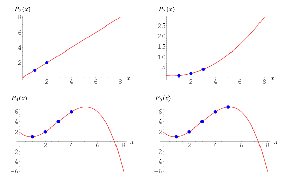
В рамках статьи предлагаю за такую функцию взять десятичный логарифм
 и следующие точки:

Представляя их на плоскости, должно получится нечто следующее:
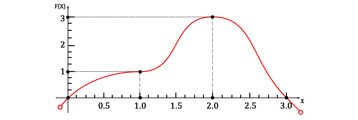
Нетрудно заметить, что сейчас кол-во пар точек равно
 .
.
При решении данной задачи приходит на ум некая системы уравнений, где кол-во линейно-независимых строк равно
. Что же это за система уравнений такая?
Давайте попробуем функцию записать в виде суммы десятичных логарифмов с коэффициентами про оных (да так, чтобы кол-во коэффициентов было равно
):

Аргументы при
различные чтобы
избежать линейной зависимости
строк в будущем (можно придумать другие). А также, учитывая, что область определения функции как минимум
![$in[0;3]$](https://habrastorage.org/getpro/habr/formulas/13f/71a/ef0/13f71aef050ab4ab1c1cf4c9d0fbb1ed.svg) (на основе заданных условием точек), мы таким образом обеспечиваем существование области значений для функции
(на основе заданных условием точек), мы таким образом обеспечиваем существование области значений для функции
в этой области определения.
Так как нам известны
пар точек, то обратимся к ним для того, чтобы построить следующую тривиальную систему:

Тривиальность системы заключается в том, что мы просто найдем такие
 , которые будет удовлетворять всему набору условия.
Собственно решая данную систему относительно
получим следующее решение:

На этом задача естественным образом подходит к концу, остается только записать это в единую функцию:

Она, разумеется, будет проходить через заданный набор точек. А график функции будет выглядеть следующим образом:
Также, ради наглядности, можно привести аппроксимированную систему решений:

Тогда аппроксимированный вид функции будет следующий:

Разумеется, никто не говорит о том, что полученная функция будет минимальной (тот же полином Лагранжа даст более короткую форму). Однако, данный метод позволяет выразить функцию через набор произвольных функций (правда, имея в виду ограничения, заданные выше по статье).
Различные примеры
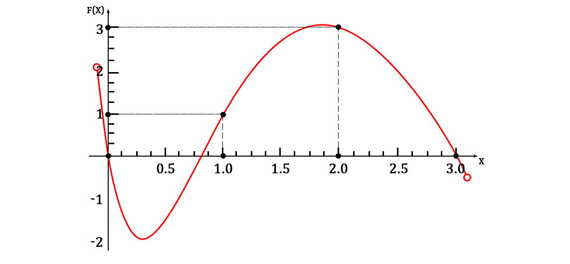
На десерт аналогично построим функцию в радикалах:

Составим систему уравнения для нахождения коэффициентов:

Её решение единственно и выглядит следующим образом:

Тогда готовая функция выглядит следующим образом:

Что по совместительтву является полином Лагранжа для данного набора точек (т.к. оный в неявном виде реализует радикальную форму алгоритма из статьи). График на области заданных точек выглядит так:
Самым интересным в данной истории является то, что произвольные функции для построения конечной функции можно
и нужно
комбинировать. Иными словами, функция может быть построена сразу на радикалах и логарифмах, а может и на чем-то другом (показательные функции, факториалы, и т.п. ). Лишь бы полученный набор функций обеспечивал линейную независимость строк при подборе коэффициентов. В общем виде для заданных
пар точек это выглядит так:

Где
 — коэффициенты которые предстоит найти через систему уравнений (СЛАУ), а
 — некоторые функции, которые обеспечат линейную независимость при нахождении коэффициентов.
А дальше — по алгоритму выше, всё совершенно аналогично. Не забывая о том, что
должны быть определены на заданных условием точках.
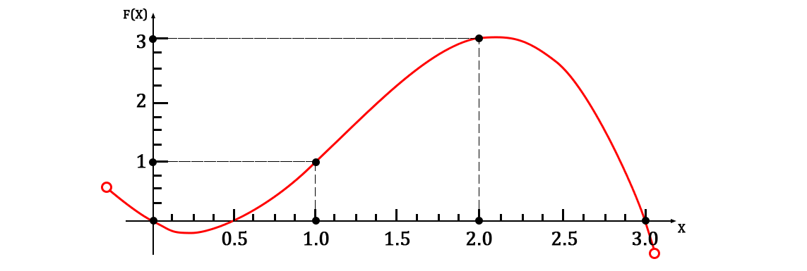
К примеру можно показать функцию, состоящую из полностью различных базовых функций:

Дабы удовлетворить заданному набору точек, коэффициенты будут в таком случае следующие (найдены строго по алгоритму из статьи):

А сама функция будет такой:

График же будет выглядит практически также как предыдущий (на области заданных точек).
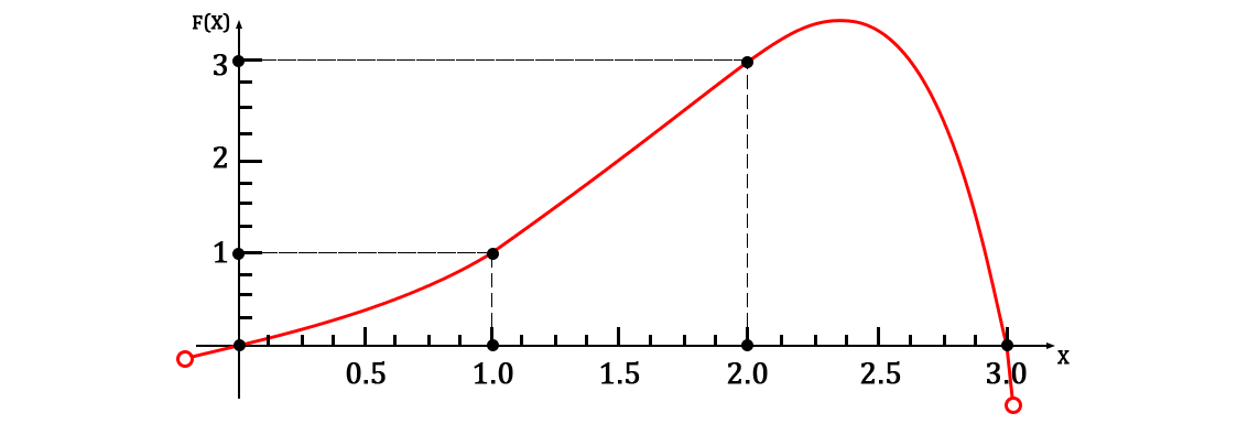
Если хочется более «гладкий» график, то можно посмотреть в сторону факториальной формы, например такой:

Найдем коэффициенты:

Подставим оные в готовую функцию:

А также полюбуемся очень хорошим графиком:
Зачем это нужно?
Да хотя бы для того, чтобы представить себе пучок веревок, стянутых пластиковыми хомутами 
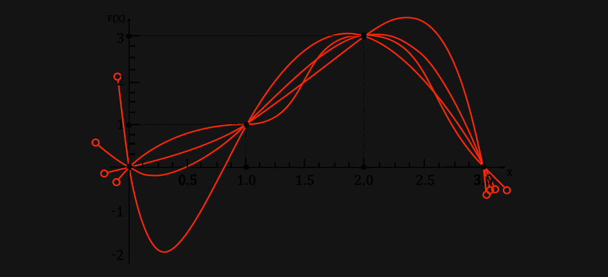
(* Тут мы просто наложили все графики друг на друга)
На этом в рамках текущей статьи все, рекомендую поиграться самостоятельно.
Всего наилучшего,
с вами был Петр.
In numerical analysis, polynomial interpolation is the interpolation of a given data set by the polynomial of lowest possible degree that passes through the points of the dataset.[1]
Given a set of n + 1 data points  , with no two
  the same, a polynomial function
  is said to interpolate the data if
  for each
  .
.
Two common explicit formulas for this polynomial are the Lagrange polynomials and Newton polynomials.
Applications[edit]
Polynomials can be used to approximate complicated curves, for example, the shapes of letters in typography,[citation needed] given a few points. A relevant application is the evaluation of the natural logarithm and trigonometric functions: pick a few known data points, create a lookup table, and interpolate between those data points. This results in significantly faster computations.[specify] Polynomial interpolation also forms the basis for algorithms in numerical quadrature and numerical ordinary differential equations and Secure Multi Party Computation, Secret Sharing schemes.
Polynomial interpolation is also essential to perform sub-quadratic multiplication and squaring such as Karatsuba multiplication and Toom–Cook multiplication, where an interpolation through points on a polynomial which defines the product yields the product itself. For example, given a = f(x) = a0x0 + a1x1 + … and b = g(x) = b0x0 + b1x1 + …, the product ab is equivalent to W(x) = f(x)g(x). Finding points along W(x) by substituting x for small values in f(x) and g(x) yields points on the curve. Interpolation based on those points will yield the terms of W(x) and subsequently the product ab. In the case of Karatsuba multiplication this technique is substantially faster than quadratic multiplication, even for modest-sized inputs. This is especially true when implemented in parallel hardware.
Interpolation theorem[edit]
There exists a unique polynomial of degree at most  that interpolates the
  data points
  , where no two are the same.[2]
Equivalently, for a fixed choice of interpolation nodes , polynomial interpolation defines a linear bijection between the n-tuples of real-number values  and the vector space
  of real polynomials of degree at most n:

This is a type of unisolvence theorem. The theorem is also valid over any infinite field in place of the real numbers  , for example the rational or complex numbers.
First proof[edit]
Consider the Lagrange basis functions given by

Notice that  is a polynomial of degree . Furthermore, for each
  we have
  , where
  is the Kronecker delta. It follows that the linear combination

is an interpolating polynomial of degree .
To prove uniqueness, assume that there exists another interpolating polynomial  of degree at most . Since
  for all
  , it follows that the polynomial
  has distinct zeros. However, is of degree at most and, by the fundamental theorem of algebra,[3] can have at most zeros; therefore,
  .
.
Second proof[edit]
Write out the interpolation polynomial in the form
|
|
(1) |

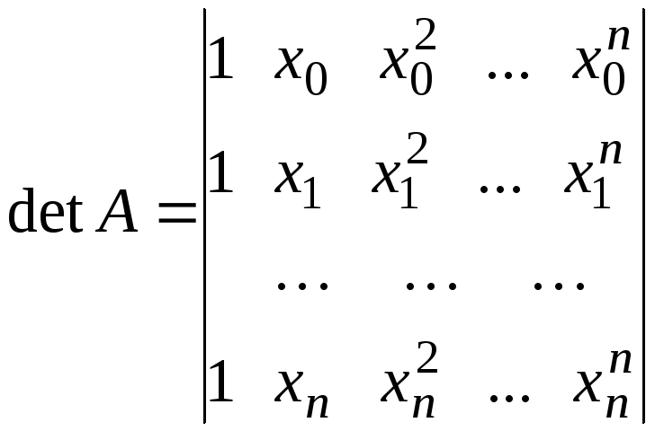
Substituting this into the interpolation equations , we get a system of linear equations in the coefficients  , which reads in matrix-vector form as the following multiplication:

An interpolant corresponds to a solution  of the above matrix equation
  . The matrix X on the left is a Vandermonde matrix, whose determinant is known to be
  which is non-zero since the nodes are all distinct. This ensures that the matrix is invertible and the equation has the unique solution
  ; that is, exists and is unique.
Corollary[edit]
If  is a polynomial of degree at most , then the interpolating polynomial of at distinct points is itself.
Constructing the interpolation polynomial[edit]
The red dots denote the data points (xk, yk), while the blue curve shows the interpolation polynomial.
The Vandermonde matrix in the second proof above may have large condition number,[4] causing large errors when computing the coefficients ai if the system of equations is solved using Gaussian elimination.
Several authors have therefore proposed algorithms which exploit the structure of the Vandermonde matrix to compute numerically stable solutions in O(n2) operations instead of the O(n3) required by Gaussian elimination.[5][6][7] These methods rely on constructing first a Newton interpolation of the polynomial and then converting it to the monomial form above.
Alternatively, we may write down the polynomial immediately in terms of Lagrange polynomials:
![{displaystyle {begin{aligned}p(x)&={frac {(x-x_{1})(x-x_{2})cdots (x-x_{n})}{(x_{0}-x_{1})(x_{0}-x_{2})cdots (x_{0}-x_{n})}}y_{0}\[4pt]&+{frac {(x-x_{0})(x-x_{2})cdots (x-x_{n})}{(x_{1}-x_{0})(x_{1}-x_{2})cdots (x_{1}-x_{n})}}y_{1}\[4pt]&+cdots \[4pt]&+{frac {(x-x_{0})(x-x_{1})cdots (x-x_{n-1})}{(x_{n}-x_{0})(x_{n}-x_{1})cdots (x_{n}-x_{n-1})}}y_{n}\[7pt]&=sum _{i=0}^{n}{Biggl (}prod _{stackrel {!0,leq ,j,leq ,n}{j,neq ,i}}{frac {x-x_{j}}{x_{i}-x_{j}}}{Biggr )}y_{i}end{aligned}}}](https://wikimedia.org/api/rest_v1/media/math/render/svg/ce5d52a889bb9e954e0814bd1545a879e2114ba8)
For matrix arguments, this formula is called Sylvester’s formula and the matrix-valued Lagrange polynomials are the Frobenius covariants.
Non-Vandermonde solutions[edit]
We are trying to construct our unique interpolation polynomial in the vector space Πn of polynomials of degree n. When using a monomial basis for Πn we have to solve the Vandermonde matrix to construct the coefficients ak for the interpolation polynomial. This can be a very costly operation (as counted in clock cycles of a computer trying to do the job). By choosing another basis for Πn we can simplify the calculation of the coefficients but then we have to do additional calculations when we want to express the interpolation polynomial in terms of a monomial basis.
One method is to write the interpolation polynomial in the Newton form and use the method of divided differences to construct the coefficients, e.g. Neville’s algorithm. The cost is O(n2) operations, while Gaussian elimination costs O(n3) operations. Furthermore, you only need to do O(n) extra work if an extra point is added to the data set, while for the other methods, you have to redo the whole computation.
Another method is to use the Lagrange form of the interpolation polynomial. The resulting formula immediately shows that the interpolation polynomial exists under the conditions stated in the above theorem. Lagrange formula is to be preferred to Vandermonde formula when we are not interested in computing the coefficients of the polynomial, but in computing the value of p(x) in a given x not in the original data set. In this case, we can reduce complexity to O(n2).[8]
The Bernstein form was used in a constructive proof of the Weierstrass approximation theorem by Bernstein and has gained great importance in computer graphics in the form of Bézier curves.
Linear combination of the given values[edit]
The Lagrange form of the interpolating polynomial is a linear combination of the given values. In many scenarios, an efficient and convenient polynomial interpolation is a linear combination of the given values, using previously known coefficients. Given a set of  data points
  where each data point is a (position, value) pair and where no two positions are the same, the interpolation polynomial in the Lagrange form is a linear combination

of the given values  with each coefficient
  given by evaluating the corresponding Lagrange basis polynomial using the given positions .

Each coefficient in the linear combination depends on the given positions and the desired position  , but not on the given values . For each coefficient, inserting the values of the given positions and simplifying yields an expression , which depends only on . Thus the same coefficient expressions can be used in a polynomial interpolation of a given second set of data points
  at the same given positions , where the second given values
  differ from the first given values . Using the same coefficient expressions as for the first set of data points, the interpolation polynomial of the second set of data points is the linear combination

For each coefficient in the linear combination, the expression resulting from the Lagrange basis polynomial  only depends on the relative spaces between the given positions, not on the individual value of any position. Thus the same coefficient expressions can be used in a polynomial interpolation of a given third set of data points

where each position  is related to the corresponding position in the first set by
  and the desired positions are related by
  , for a constant scaling factor a and a constant shift b for all positions. Using the same coefficient expressions
  as for the first set of data points, the interpolation polynomial of the third set of data points is the linear combination

In many applications of polynomial interpolation, the given set of data points is at equally spaced positions. In this case, it can be convenient to define the x-axis of the positions such that  . For example, a given set of 3 equally-spaced data points
  is then
  .
.
The interpolation polynomial in the Lagrange form is the linear combination

This quadratic interpolation is valid for any position x, near or far from the given positions. So, given 3 equally-spaced data points at  defining a quadratic polynomial, at an example desired position
  , the interpolated value after simplification is given by
This is a quadratic interpolation typically used in the Multigrid method. Again given 3 equally-spaced data points at defining a quadratic polynomial, at the next equally spaced position  , the interpolated value after simplification is given by

In the above polynomial interpolations using a linear combination of the given values, the coefficients were determined using the Lagrange method. In some scenarios, the coefficients can be more easily determined using other methods. Examples follow.
According to the method of finite differences, for any polynomial of degree d or less, any sequence of  values at equally spaced positions has a
  th difference exactly equal to 0. The element sd+1 of the Binomial transform is such a th difference. This area is surveyed here.[9] The binomial transform, T, of a sequence of values {vn}, is the sequence {sn} defined by

Ignoring the sign term  , the coefficients of the element sn are the respective elements of the row n of Pascal’s Triangle. The triangle of binomial transform coefficients is like Pascal’s triangle. The entry in the nth row and kth column of the BTC triangle is
  for any non-negative integer n and any integer k between 0 and n. This results in the following example rows n = 0 through n = 7, top to bottom, for the BTC triangle:
| 1 | Row n = 0 | |||||||||||||||
| 1 | −1 | Row n = 1 or d = 0 | ||||||||||||||
| 1 | −2 | 1 | Row n = 2 or d = 1 | |||||||||||||
| 1 | −3 | 3 | −1 | Row n = 3 or d = 2 | ||||||||||||
| 1 | −4 | 6 | −4 | 1 | Row n = 4 or d = 3 | |||||||||||
| 1 | −5 | 10 | −10 | 5 | −1 | Row n = 5 or d = 4 | ||||||||||
| 1 | −6 | 15 | −20 | 15 | −6 | 1 | Row n = 6 or d = 5 | |||||||||
| 1 | −7 | 21 | −35 | 35 | −21 | 7 | −1 | Row n = 7 or d = 6 | ||||||||
For convenience, each row n of the above example BTC triangle also has a label  . Thus for any polynomial of degree d or less, any sequence of values at equally spaced positions has a linear combination result of 0, when using the elements of row d as the corresponding linear coefficients.
For example, 4 equally spaced data points of a quadratic polynomial obey the linear equation given by row  of the BTC triangle.
  This is the same linear equation as obtained above using the Lagrange method.
The BTC triangle can also be used to derive other polynomial interpolations. For example, the above quadratic interpolation

can be derived in 3 simple steps as follows. The equally spaced points of a quadratic polynomial obey the rows of the BTC triangle with or higher. First, the row  spans the given and desired data points
  with the linear equation

Second, the unwanted data point  is replaced by an expression in terms of wanted data points. The row provides a linear equation with a term
  , which results in a term
  by multiplying both sides of the linear equation by 4.

Third, the above two linear equations are added to yield a linear equation equivalent to the above quadratic interpolation for  .
.

Similar to other uses of linear equations, the above derivation scales and adds vectors of coefficients. In polynomial interpolation as a linear combination of values, the elements of a vector correspond to a contiguous sequence of regularly spaced positions. The p non-zero elements of a vector are the p coefficients in a linear equation obeyed by any sequence of p data points from any degree d polynomial on any regularly spaced grid, where d is noted by the subscript of the vector. For any vector of coefficients, the subscript obeys  . When adding vectors with various subscript values, the lowest subscript applies for the resulting vector. So, starting with the vector of row and the vector of row of the BTC triangle, the above quadratic interpolation for is derived by the vector calculation

Similarly, the cubic interpolation typical in the Multigrid method,

can be derived by a vector calculation starting with the vector of row  and the vector of row of the BTC triangle.

Interpolation error[edit]
When interpolating a given function f by a polynomial  of degree n at the nodes x0,…, xn we get the error
![{displaystyle f(x)-p_{n}(x)=f[x_{0},ldots ,x_{n},x]prod _{i=0}^{n}(x-x_{i})}](https://wikimedia.org/api/rest_v1/media/math/render/svg/20e8c5d91ab5d500891ea9c0b0b528881dde5b08)
where
![{displaystyle f[x_{0},ldots ,x_{n},x]}](https://wikimedia.org/api/rest_v1/media/math/render/svg/19168012592a247cadfadee2ec1a0329c5288f1f)
is the notation for divided differences.
If f is n + 1 times continuously differentiable on a closed interval I and is a polynomial of degree at most n that interpolates f at n + 1 distinct points {xi} (i = 0, 1,…, n) in that interval, then for each x in the interval there exists ξ in that interval such that

The above error bound suggests choosing the interpolation points xi such that the product  is as small as possible. The Chebyshev nodes achieve this.
Proof[edit]
Set the error term as

and set up an auxiliary function:

where

Since xi are roots of  and
and  , we have Y(x) = Y(xi) = 0, which means Y has at least n + 2 roots. From Rolle’s theorem,
  has at least n + 1 roots, then
  has at least one root ξ, where ξ is in the interval I.
So we can get

Since  is a polynomial of degree at most n, then

Thus

Since ξ is the root of , so

Therefore,

Thus the remainder term in the Lagrange form of the Taylor theorem is a special case of interpolation error when all interpolation nodes xi are identical.[10] Note that the error will be zero when  for any i. Thus, the maximum error will occur at some point in the interval between two successive nodes.
For equally spaced intervals[edit]
In the case of equally spaced interpolation nodes where  , for
, for  and where
  the product term in the interpolation error formula can be bound as[11]

Thus the error bound can be given as
![{displaystyle left|R_{n}(x)right|leq {frac {h^{n+1}}{4(n+1)}}max _{xi in [a,b]}left|f^{(n+1)}(xi )right|}](https://wikimedia.org/api/rest_v1/media/math/render/svg/34dc247e57d4dcc78f9484b320ed389b1ddb375c)
However, this assumes that  is dominated by
  , i.e.
  . In several cases, this is not true and the error actually increases as n → ∞ (see Runge’s phenomenon). That question is treated in the section Convergence properties.
Lebesgue constants[edit]
We fix the interpolation nodes x0, …, xn and an interval [a, b] containing all the interpolation nodes. The process of interpolation maps the function f to a polynomial p. This defines a mapping X from the space C([a, b]) of all continuous functions on [a, b] to itself. The map X is linear and it is a projection on the subspace Πn of polynomials of degree n or less.
The Lebesgue constant L is defined as the operator norm of X. One has (a special case of Lebesgue’s lemma):

In other words, the interpolation polynomial is at most a factor (L + 1) worse than the best possible approximation. This suggests that we look for a set of interpolation nodes that makes L small. In particular, we have for Chebyshev nodes:

We conclude again that Chebyshev nodes are a very good choice for polynomial interpolation, as the growth in n is exponential for equidistant nodes. However, those nodes are not optimal.
Convergence properties[edit]
It is natural to ask, for which classes of functions and for which interpolation nodes the sequence of interpolating polynomials converges to the interpolated function as n → ∞? Convergence may be understood in different ways, e.g. pointwise, uniform or in some integral norm.
The situation is rather bad for equidistant nodes, in that uniform convergence is not even guaranteed for infinitely differentiable functions. One classical example, due to Carl Runge, is the function f(x) = 1 / (1 + x2) on the interval [−5, 5]. The interpolation error || f − pn||∞ grows without bound as n → ∞. Another example is the function f(x) = |x| on the interval [−1, 1], for which the interpolating polynomials do not even converge pointwise except at the three points x = ±1, 0.[12]
One might think that better convergence properties may be obtained by choosing different interpolation nodes. The following result seems to give a rather encouraging answer:
Theorem — For any function f(x) continuous on an interval [a,b] there exists a table of nodes for which the sequence of interpolating polynomials converges to f(x) uniformly on [a,b].
Proof
It is clear that the sequence of polynomials of best approximation  converges to f(x) uniformly (due to the Weierstrass approximation theorem). Now we have only to show that each may be obtained by means of interpolation on certain nodes. But this is true due to a special property of polynomials of best approximation known from the equioscillation theorem. Specifically, we know that such polynomials should intersect f(x) at least n + 1 times. Choosing the points of intersection as interpolation nodes we obtain the interpolating polynomial coinciding with the best approximation polynomial.
The defect of this method, however, is that interpolation nodes should be calculated anew for each new function f(x), but the algorithm is hard to be implemented numerically. Does there exist a single table of nodes for which the sequence of interpolating polynomials converge to any continuous function f(x)? The answer is unfortunately negative:
Theorem — For any table of nodes there is a continuous function f(x) on an interval [a, b] for which the sequence of interpolating polynomials diverges on [a,b].[13]
The proof essentially uses the lower bound estimation of the Lebesgue constant, which we defined above to be the operator norm of Xn (where Xn is the projection operator on Πn). Now we seek a table of nodes for which
![{displaystyle lim _{nto infty }X_{n}f=f,{text{ for every }}fin C([a,b]).}](https://wikimedia.org/api/rest_v1/media/math/render/svg/dee3b117b4b32fbb477a4ffb88e213b0177e9b25)
Due to the Banach–Steinhaus theorem, this is only possible when norms of Xn are uniformly bounded, which cannot be true since we know that

For example, if equidistant points are chosen as interpolation nodes, the function from Runge’s phenomenon demonstrates divergence of such interpolation. Note that this function is not only continuous but even infinitely differentiable on [−1, 1]. For better Chebyshev nodes, however, such an example is much harder to find due to the following result:
Theorem — For every absolutely continuous function on [−1, 1] the sequence of interpolating polynomials constructed on Chebyshev nodes converges to f(x) uniformly.[14]
[edit]
Runge’s phenomenon shows that for high values of n, the interpolation polynomial may oscillate wildly between the data points. This problem is commonly resolved by the use of spline interpolation. Here, the interpolant is not a polynomial but a spline: a chain of several polynomials of a lower degree.
Interpolation of periodic functions by harmonic functions is accomplished by Fourier transform. This can be seen as a form of polynomial interpolation with harmonic base functions, see trigonometric interpolation and trigonometric polynomial.
Hermite interpolation problems are those where not only the values of the polynomial p at the nodes are given, but also all derivatives up to a given order. This turns out to be equivalent to a system of simultaneous polynomial congruences, and may be solved by means of the Chinese remainder theorem for polynomials. Birkhoff interpolation is a further generalization where only derivatives of some orders are prescribed, not necessarily all orders from 0 to a k.
Collocation methods for the solution of differential and integral equations are based on polynomial interpolation.
The technique of rational function modeling is a generalization that considers ratios of polynomial functions.
At last, multivariate interpolation for higher dimensions.
See also[edit]
- Newton series
- Polynomial regression
Notes[edit]
- ^ Tiemann, Jerome J. (May–June 1981). «Polynomial Interpolation». I/O News. 1 (5): 16. ISSN 0274-9998. Retrieved 3 November 2017.
- ^ Humpherys, Jeffrey; Jarvis, Tyler J. (2020). «9.2 — Interpolation». Foundations of Applied Mathematics Volume 2: Algorithms, Approximation, Optimization. Society for Industrial and Applied Mathematics. p. 418. ISBN 978-1-611976-05-2.
- ^ Humpherys, Jeffrey; Jarvis, Tyler J.; Evans, Emily J. (2017). «15.3: The Fundamental Theorem of Arithmetic». Foundations of Applied Mathematics Volume 1: Mathematical Analysis. Society for Industrial and Applied Mathematics. p. 591. ISBN 978-1-611974-89-8.
- ^ Gautschi, Walter (1975). «Norm Estimates for Inverses of Vandermonde Matrices». Numerische Mathematik. 23 (4): 337–347. doi:10.1007/BF01438260. S2CID 122300795.
- ^ Higham, N. J. (1988). «Fast Solution of Vandermonde-Like Systems Involving Orthogonal Polynomials». IMA Journal of Numerical Analysis. 8 (4): 473–486. doi:10.1093/imanum/8.4.473.
- ^ Björck, Å; V. Pereyra (1970). «Solution of Vandermonde Systems of Equations». Mathematics of Computation. American Mathematical Society. 24 (112): 893–903. doi:10.2307/2004623. JSTOR 2004623.
- ^ Calvetti, D.; Reichel, L. (1993). «Fast Inversion of Vandermonde-Like Matrices Involving Orthogonal Polynomials». BIT. 33 (3): 473–484. doi:10.1007/BF01990529. S2CID 119360991.
- ^ R.Bevilaqua, D. Bini, M.Capovani and O. Menchi (2003). Appunti di Calcolo Numerico. Chapter 5, p. 89. Servizio Editoriale Universitario Pisa — Azienda Regionale Diritto allo Studio Universitario.
- ^ Boyadzhiev, Boyad (2012). «Close Encounters with the Stirling Numbers of the Second Kind» (PDF). Math. Mag. 85 (4): 252–266. arXiv:1806.09468. doi:10.4169/math.mag.85.4.252. S2CID 115176876.
- ^ «Errors in Polynomial Interpolation» (PDF).
- ^ «Notes on Polynomial Interpolation» (PDF).
- ^ Watson (1980, p. 21) attributes the last example to Bernstein (1912).
- ^ Watson (1980, p. 21) attributes this theorem to Faber (1914).
- ^ Krylov, V. I. (1956). «Сходимость алгебраического интерполирования покорням многочленов Чебышева для абсолютно непрерывных функций и функций с ограниченным изменением» [Convergence of algebraic interpolation with respect to the roots of Chebyshev’s polynomial for absolutely continuous functions and functions of bounded variation]. Doklady Akademii Nauk SSSR. New Series (in Russian). 107: 362–365. MR 18-32.
References[edit]
- Bernstein, Sergei N. (1912). «Sur l’ordre de la meilleure approximation des fonctions continues par les polynômes de degré donné» [On the order of the best approximation of continuous functions by polynomials of a given degree]. Mem. Acad. Roy. Belg. (in French). 4: 1–104.
- Faber, Georg (1914). «Über die interpolatorische Darstellung stetiger Funktionen» [On the Interpolation of Continuous Functions]. Deutsche Math. Jahr. (in German). 23: 192–210.
- Watson, G. Alistair (1980). Approximation Theory and Numerical Methods. John Wiley. ISBN 0-471-27706-1.
Further reading[edit]
- Atkinson, Kendell A. (1988). «Chapter 3.». An Introduction to Numerical Analysis (2nd ed.). John Wiley and Sons. ISBN 0-471-50023-2.
- Brutman, L. (1997). «Lebesgue functions for polynomial interpolation — a survey». Ann. Numer. Math. 4: 111–127.
- Powell, M. J. D. (1981). «Chapter 4». Approximation Theory and Methods. Cambridge University Press. ISBN 0-521-29514-9.
- Schatzman, Michelle (2002). «Chapter 4». Numerical Analysis: A Mathematical Introduction. Oxford: Clarendon Press. ISBN 0-19-850279-6.
- Süli, Endre; Mayers, David (2003). «Chapter 6». An Introduction to Numerical Analysis. Cambridge University Press. ISBN 0-521-00794-1.
External links[edit]
- «Interpolation process», Encyclopedia of Mathematics, EMS Press, 2001 [1994]
- ALGLIB has an implementations in C++ / C#.
- GSL has a polynomial interpolation code in C
- Polynomial Interpolation demonstration.
225
Глава 4. Многочленная
интерполяция
Большая
часть численных методов позволяет
получать не точные, а приближенные
решения математических задач. Поэтому
очень важной в вычислительной математике
является задача приближения (аппроксимации)
различных математических объектов.
Чаще всего приближаются (аппроксимируются)
функции. А один из самых распространенных
способов аппроксимации функций –
интерполирование. Оно используется в
тех случаях, когда основная информация
о приближаемой функции дается в виде
таблицы ее значений, а табличные значения
имеют незначительные погрешности.
4.1.Интерполяционный многочлен Лагранжа Постановка задачи интерполирования
Пусть
функция
![]() определена на заданном отрезке
определена на заданном отрезке![]() .
.
Известны значения функции![]() в отдельных точках
в отдельных точках![]() (
(![]() )
)
этого отрезка. Вычисление значений
этой функции в других точках отрезка![]() либо очень трудоемко, либо вообще
либо очень трудоемко, либо вообще
невозможно. В таких условиях обычно
стараются получить приближение для
функции![]() ,
,
которым можно было бы воспользоваться
для вычисления приближенных значений
функции в других точках отрезка![]() или для других целей.Под
или для других целей.Под
приближением функции
![]() на
на
отрезке
![]() понимается
понимается
некоторая другая функция
![]() ,определенная
,определенная
на этом
отрезке
![]() ,значения
,значения
которой достаточно близки к соответствующим
значениям функции
![]()
![]() .
.
При
построении приближений для функций с
известной таблицей значений используется
несколько способов. Самый распространенный
из них называется интерполяцией.
При интерполяции от приближения
требуется, чтобы оно имело ту же таблицу
значений, что и приближаемая функция:
![]() ,
,
![]() .
.
(4.1.1)
Это
условие получило название условия
интерполяции.
Функция
![]() ,удовлетворяющая
,удовлетворяющая
условиям интерполяции, называется
интерполяционной,
а точки
![]()
узлами
интерполяции.
Чаще
всего в качестве интерполяционных
функций выбирают алгебраические
многочлены, поскольку их значения проще
всего вычисляются. В результате возникает
следующая задача.
Задача многочленной интерполяции. Ищется алгебраический многочлен n-й степени , удовлетворяющий условиям интерполяции
![]() .
.
(4.1.2)
Алгебраический
многочлен, удовлетворяющий условиям
(4.1.2), называется интерполяционным
многочленом.
При записи интерполяционного многочлена
будем использовать также более развернутое
обозначение
![]() ,
,
в котором указываются узлы интерполяции
в качествепараметров.
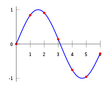
Геометрический
смысл интерполяции
состоит в том, что графики функции
![]() и интерполяционного многочлена
и интерполяционного многочлена![]() должны проходить через все табличные
должны проходить через все табличные
точки![]() ,
,
(![]() ).
).
На рис. 4.1 эти точки выделены. Именно это
условие должно обеспечить близость
графиков этих функций на отрезке![]() ,
,
чтобы можно было использовать
интерполяционный многочлен![]()
![]() в
в
качестве приближения для функции![]() .
.
И
 Рис.
Рис.
4.1
нтуитивно понятно, что если табличных
точек![]() будет много и они будут расположены
будет много и они будут расположены
густо, то графики функции![]() и интерполяционного многочлена
и интерполяционного многочлена![]() будут расположены близко друг к другу.
будут расположены близко друг к другу.
Обычно
постановка любой прикладной математической
задачи подразумевает исследование
существования и единственности
ее решения.
Поэтому далее займемся этими вопросами
в отношении задачи
многочленной интерполяции.
Будем
искать решение задачи интерполяции в
виде
![]()
![]() .
.
(4.1.3)
Требуется
определить набор постоянных (![]() )
)
таким образом, чтобы алгебраический
многочлен (4.1.3) удовлетворял условию
интерполяции (4.1.2). Для этого подставим
формулу (4.1.3) в формулу (4.1.2):
 (4.1.4)
Система
(4.1.4) представляет собой систему линейных
алгебраических уравнений с постоянными
коэффициентами относительно неизвестных
постоянных
![]() .
.
Определитель матрицы этой системы
хорошо
известен и получил название определителя
Вандермонда.
Доказано, что если все узлы интерполяции
![]() попарно различны, то определительВандермонда
попарно различны, то определительВандермонда
не равен нулю.
Таким образом, система
(4.1.4) должна иметь единственное решение,
если все
![]()
попарно различны.
Обозначим это решение
![]() .
.
Подставляя координаты этого вектора в
формулу (4.1.3), получим интерполяционный
многочлен в виде
![]()
![]() .
.
(4.1.5)
Таким
образом, доказано существование и
единственность интерполяционного
многочлена, если все узлы интерполяции
попарно различны. На этом постановку
задачи многочленной интерполяции
закончим. Фактически мы не только
поставили эту задачу, но и получили
метод ее решения, сведя задачу интерполяции
к задаче решения линейной системы.
Соседние файлы в папке ВМ_УЧЕБНИК
- #
- #
- #
- #
- #
- #
- #
- #
- #
- #
- #
Экстраполяцией называется построение математических моделей, предсказывающих значения вне некоторого известного промежутка — например, следующее значение по известным предыдущим.
Интерполяцией же называется приближенное нахождение промежуточных значений между известными.
В более узком смысле, в контексте алгебры, интерполяцией называется нахождение многочлена, проходящего через заданный набор точек $(x_i, y_i)$.
#Интерполяционный многочлен Лагранжа
Теорема. Пусть есть набор различных точек $x_0, x_1, dots, x_{n}$. Многочлен степени $n$ однозначно задаётся своими значениями в этих точках.
Примечание: коэффициентов у этого многочлена столько же, сколько и точек.
Доказательство будет конструктивным — можно явным образом задать многочлен, который принимает заданные значения $y_0, y_1, ldots, y_n$ в этих точках:
$$
y(x)=sumlimits_{i=0}^{n}y_iprodlimits_{jneq i}dfrac{x-x_j}{x_i-x_j}
$$
Этот многочлен называется интерполяционным многочленом Лагранжа.
Корректность. Проверим, что в точке $x_i$ значение действительно будет равно $y$:
-
Для $i$-го слагаемого внутреннее произведение будет равно единице, если вместо $x$ подставить $x_i$: в этом случае просто перемножается $(n-1)$ единица. Эта единица помножится на $y_i$ и войдёт в сумму.
-
Для всех остальных слагаемых произведение занулится: один из множителей будет равен $(x_i — x_i)$.
Уникальность. Предположим, есть два подходящих многочлена степени $n$: $A(x)$ и $B(x)$. Рассмотрим их разность. В точках $x_i$ значение получившегося многочлена $A(x) — B(x)$ будет равняться нулю. Если так, то точки $x_i$ должны являться его корнями, и тогда разность можно записать так:
$$
A(x) — B(x) = alpha prod_{i=0}^n (x-x_i)
$$
для какого-то числа $alpha$. Тут мы получаем противоречие: если раскрыть это произведение, то получится многочлен степени $n+1$, который нельзя получить разностью двух многочленов степени $n$.
#Интерполяция на практике
Примечание. На практике интерполяцию решают методом Гаусса: её можно свести к решению линейного уравнения $aX = y$, где $X$ это матрица следующего вида:
$$
begin{pmatrix}
1 & x_0 & x_0^2 & ldots & x_0^n \
1 & x_1 & x_1^2 & ldots & x_1^n \
vdots & vdots & vdots & ddots & vdots \
1 & x_n & x_n^2 & ldots & x_n^n \
end{pmatrix}
$$
Важный факт — многочлен степени $n$ можно однозначно задать
- своими $(n+1)$ коэффициентами,
- значениями хотя бы в $(n + 1)$ точке,
- своими $n$ корнями (возможно, комплексными и дублирующимися) и коэффициентом $alpha$:
$$
A(x) = alpha prod (x-x_i)^{k_i}
$$
Последнее утверждение (что у любого многочлена существует $n$ комплексных корней) называется основной теоремой алгебры, и его доказательство выходит немного за пределы этой статьи.
Интерполяцио́нный многочле́н Лагра́нжа — многочлен минимальной степени, принимающий данные значения в данном наборе точек. Для пар чисел  , где все
  различны, существует единственный многочлен
  степени не более , для которого
  .
.
В простейшем случае  это линейный многочлен, график которого — прямая, проходящая через две заданные точки.
Определение
Файл:Lagrangepolys.png Этот пример показывает интерполяционный многочлен Лагранжа для четырёх точек (-9,5), (-4,2), (-1,-2) и (7,9), а также полиномы yj lj(x), каждый из которых проходит через одну из выделенных точек, и принимает нулевое значение в остальных xi
Лагранж предложил способ вычисления таких многочленов:

где базисные полиномы определяются по формуле:

Легко видеть что  обладают такими свойствами:
Отсюда следует, что , как линейная комбинация , может иметь степень не больше , и  , Q.E.D.
Применения
Полиномы Лагранжа используются для интерполяции, а также для
численного интегрирования.
Пусть для функции  известны значения
  в некоторых точках. Тогда мы можем интерполировать эту функцию как

В частности,

Значения интегралов от  не зависят от , и их можно вычислить заранее, зная последовательность .
Для случая равномерного распределения по отрезку узлов интерполяции
В указанном случае можно выразить через расстояние между узлами интерполяции h и начальную точку  :
:
 ,
,

и, следовательно,
- .

Подставив эти выражения в формулу полинома и вынеся h за знаки перемножения в числителе и знаменателе, получим

Теперь можно ввести замену переменной

и получить полином от XY, который строится с использованием только целочисленной арифметики. Недостатком данного подхода является факториальная сложность числителя и знаменателя, что требует использования алгоритмов с многобайтным представлением чисел.
cs:Lagrangeova interpolace
nl:Lagrange-polynoom
sr:Лагранжов полином
uk:Многочлен Лагранжа