Как найти характеристическую функцию случайной величины

Характеристическая функция случайной величины

Для случайной величины $xi$ характеристическая функция (ХФ) определяется следующим образом:

$$
phi_{xi}(t)=M[e^{i txi}].
$$

Для дискретной случайной величины с законом вида $(x_k,p_k)$ характеристическая функция выражается как

$$phi_{xi}(t)=M[e^{i txi}]=sum_k e^{i t x_k}cdot p_k.$$

Для непрерывной случайной величины с плотностью распределения $f(x)$:

$$phi_{xi}(t)=M[e^{i txi}]=int_{-infty}^{infty} e^{itx}cdot f(x),dx.$$

Характеристическая функция — это преобразование Фурье распределения случайной
величины.

По известной характеристической функции можно вычислять моменты случайной величины по формуле:

$$M[xi^n] = frac{1}{i^n} cdotfrac{d^n}{dx^n} phi_{xi}(t)|_{t=0}. $$

Характеристическая функция однозначно определяет распределение случайной величины. ХФ суммы независимых случайных величин равна произведению их характеристических функций (это свойство используется для доказательства композиционной устойчивости, например в примере 3 для нормального распределения). ХФ существует всегда, непрерывна, ограничена ($|phi_{xi}(t)| le 1$), в нуле равна единице.

В этом разделе вы найдете примеры нахождения характеристической функции и моментов для разных законов распределения.

Полезная страница? Сохрани или расскажи друзьям

Примеры решений: характеристическая функция

Задача 1. По заданному закону или плотности распределения случайной величины $xi$ найти характеристическую функцию $phi(t)$.
Закон Пуассона: $$P(xi=k)=a^k/k!cdot e^{-a}, k=1,2,… a=0.38$$

Задача 2. По заданному закону распределения найти характеристическую функцию $phi(t)$, кумулянтную функцию $gamma(t)$ и первые четыре семиинварианта этого распределения.
Биномиальный закон (Бернулли)

$$P(xi=k)=C_n^k p^k (1-p)^{n-k}, 0 lt p lt 1, k=0,1,2,…,n.$$

Задача 3. С помощью характеристических функций, доказать, что сумма независимых нормально распределенных случайных величин имеет нормальное распределение. Указать параметры этого распределения.

Задача 4. Найти характеристическую функцию дискретной случайной величины Х, подчиняющейся закон распределения Паскаля $P(X=m)=a^m/(1+a)^{m+1} (agt 0)$. По ней найти $M[X]$ и $D[X]$.

Задача 5. Найти характеристическую функцию непрерывной случайной величины, имеющей плотность распределения $p_{xi}(x)=e^{-|x|}/2.$

Мы отлично умеем решать задачи по теории вероятностей

Источник

3.1. Характеристическая функция биномиального закона.

Пусть с.в.
,
распределена по биномиальному закону.
Найти,
а затем выразить,,
через.
Имеет место утверждение.

Теорема 13.5. Для характеристической
функции
д.с.в.,
распределённой по биномиальному закону
справедлива формула

(17)
.

Доказательство.По определению
случайная величинапринимает
целочисленные значенияс вероятностями.
На основании формулы (9) и формулы бинома
Ньютона, находим

и с
учётом
,
равенство (17) доказано.

Упражнение. Для математического
ожидания и дисперсии биномиального
распределения и при любом целом,вывести на основании равенства (12)
формулы:

3.2. Характеристическая функция закона Пуассона.

Теорема 13.6. Для характеристической
функции
д.с.в.,
распределённой по закону Пуассона
справедлива формула

(18)
.

Доказательство. Согласно условию
теоремы с.в.принимает
только неотрицательные целые значения,
при этом

Найдём
характеристическую функцию с.в.

Следовательно, теорема доказана.

Упражнение. Для математического
ожидания и дисперсии распределения
Пуассона при любом целом,
ина основании равенства (12) – (15) вывести
формулы:

1.2.

Рассмотрим следующую
теоретическую задачу, которая раскрывает
ещё одну сторону закона Пуассона, где
распределение происходит с параметром,
равным произведению
.

Задача
[см. Бородин]. Число
космических частиц, попадающих в
аппаратный отсек ракеты за время её
полёта распределено по закону Пуассона
с параметром
.
При этом условная вероятность для каждой
из этих частиц попасть в уязвимый блок
равна.

Найти закон распределения
количества частиц, попадающих в уязвимый
блок.

Решение. Пусть

обозначает уязвимый блок ракеты, авыражает наступление события, когда в
уязвимый блок ракеты попалочастиц,
иобозначает аппаратный отсек ракеты, авыражает наступления событий, когда в
аппаратный отсек ракеты попалочастиц.
Тогда события,,
составляют полную группу событий, по
формуле полной вероятностии с учётом того, что для,
имеем

Далее, т.к. вероятности
гипотез согласно условию задачи равны

,
а для случаев
,
величинаопределяется
по биномиальному закону с вероятностью
«успеха» (частица попала в уязвимый
блок).
Поэтому, согласно формуле,Таким образом, окончательно получим

отсюда
на основании значения биномиальных
коэффициентов
,
получим

Таким образом, количество частиц,
попадающих в уязвимых блок ракеты также
распределены по закону Пуассона, но с
параметром, равным произведению
.

Напомним, что аналогичными формулами
мы раньше встречались в пунктах 6.2. и
9.2. в связи вероятностью наступления
потока события в случайные моменты
времени (простейшие потоки событий).

3.3. Характеристическая функция геометрического закона.

Пусть проводится неограниченное число
независимых одинаковых испытаний, в
каждом из которых событие
наступает с вероятностьюи пустьобозначает
с.в. , равная числу испытаний до момента
первого наступления события.
Тогда эта вероятность как мы уже знаем
(см. п.9.3.) равна

Это распределение называется
геометрическим,так как вероятность,
как числовая последовательность образуют
геометрическую прогрессию. Тогда
вероятность того, что событиенаступит не раньше момента,
задаётся формулой

Так как производящая функция данного
распределения (см.п.8.8.) равна
,
то согласно равенству (10) длябудем иметь

Упражнение. Для математического
ожидания и дисперсии геометрического
закона распределения на основании
формул (12) – (15) вывести равенства:

1.2.

3.4. Характеристическая
функция равномерного закона.

Вспомним, что равномерное распределение
для любых вещественных чисел
задается плотностью

Характеристическая функция равномерного
распределения вычисляется следующим
образом:

В частности, для центрально —
симметрического отрезка
получим

Следствие 4. В частности, справедливы
равенства

Упражнение. Для математического
ожидания и дисперсии равномерного
распределения на основании формул (12)
– (15) вывести равенства:

1.2.

Для случаявывести формулы:3. 4.

3.5. Характеристическая
функция показательного закона.

Как было показано в.9.6. плотность с.в.
,
распределённая по показательному закону

имеет
вид:

Характеристическая
функция показательного распределения
вычисляется следующим образом:

Упражнение. Для математического
ожидания и дисперсии показательного
распределения на основании формул (12)
– (15) вывести равенства:

1.2.

3.6. Характеристическая
функция нормального закона ().

Теорема 13.7. Для характеристической
функции
с.в.,
распределённой по нормальному закону
справедлива формула

(19)
.

Доказательство.Согласно формулы
(29), пункта 9.9 функция плотности с.в.определена равенством

Характеристическая
функция нормального распределения
вычисляется следующим образом:

Воспользуемся
интегралом Пуассона
,
в итоге для характеристической функции
с.в.
получим равенство

Следствие 5. Для целых значений
и
всех значения параметрасправедлива формула

Пример 1. Для математического
ожидания и дисперсии с.в.,
на основании формул (12) – (15) выведем
равенства:

1..

2.=.

Применим
формулу (12):

1.,
т.е..

т.е.
Получили
известные нам результаты. Следовательно,
с учётом с.к.о.эти параметры полностью определяют
случайные величины, распределённые по
нормальному закону.

Из рассмотренных примеров на предмет
нахождения характеристических функций
случайных величин (дискретных и
непрерывных) непосредственно следует,
что по законам распределения и функциям
плотности, а следовательно, по функциям
распределения с.в.
всегда
можно найти её характеристическую
функцию.

Оказывается, имеет место и обратное
предположение: а именно по характеристической
функции однозначно определяется функция
распределения. Рассмотрим ещё два
утверждения, относящиеся к формулам
«обращения и единственности».

Теорема 13.8 (формулы обращения).
Справедливы следующие утверждения:

1.Если с.в.
принимает
целочисленные значениято

(20)

где
мнимая
единица,.

2. Если характеристическая
функция
случайной величиныабсолютно интегрируема, то существует
плотности распределенияопределяемая формулой

(21)
.

Доказательство. Заметим, что для
любого целого числаи вещественногоимеют
место равенства

(22)

Действительно, пусть
любое вещественное число. Дляравенство очевидно. При любомимеем

где мы
воспользовались равенством

Используя наше равенство для случая
,
исогласно, определению характеристической
функции с.в.с
целыми значениями, получим (с учётом
того, что для отрицательных индексов
вероятностиопределены)

Тем самым первый пункт теоремы доказан.
Перейдём к доказательству второго
пункта.

Так как функция
абсолютно интегрируема, то для любыхс учётом формулы (22) имеем

(23)
.

Используя
определение характеристической функции
(см. формулу (11)),
получим

(24)

(23)
.

Используя
определение характеристической функции
(см. формулу (11)),
получим

(24)

На основании значения интеграла Дирихле
(см. Лекции по математ. анализ Архипов
и др. гл. 17. Лекция 20.)

где функция определяется равенствами:

Следовательно, получим равенства

Поэтому,
по отдельности рассматривая случаи
и

,
получим

Пусть
иточки
непрерывности функции.
Тогда приправая часть равенства (24)

стремится к равенству

Учитывая это равенство и на основании
(23) и (24), имеем

(25)
.

Поскольку функция распределения
непрерывна слева, то с помощью предельного
перехода из последовательности точек
непрерывности
ифункцииравенство
(25) распространяется на произвольные
точкии.
Теперь из (25) по определению следует,
чтоявляется плотностью функции распределении.
В итоге, из равенства (23) получим
предельное равенство.

В точках
инепрерывности
функциисправедливо
равенство

(26)
.

Равенство
(26) носит название «формулы обращения».
Она используется для вывода весьма
важного утверждения —теорема
единственности.

Упражнение. Пустьнатуральное
число,целое число. Докажите, что

справедливы
равенства

Теорема 13. 9 (единственности).
Функция распределения однозначно
определяется своей характеристической
функцией.

Доказательство. Действительно, из
равенства (26) непосредственно следует,
что в каждой точке непрерывности функцииприменима формула

В
последнем интеграле предел относительноберётся относительно множеству точекявляющихся точками непрерывности
функции.

Рассмотрим некоторые примеры приложения
последней теоремы.

Пример 2. Пусть независимые случайные
величиныираспределены по закону Пуассона, причём

Покажем,
что с.в.
распределена по закону Пуассона с
параметром.

В теореме 13.6 мы показали, что (см. (18))
.
Отсюда имеем

В силу
теоремы 13.6. характеристическая функция
суммы с.в.
равна

т.е. является характеристической функцией
некоторого закона Пуассона. Согласно
теореме 13.9 единственное распределение,
имеющее
своей характеристической функцией,
есть закон Пуассона, для которой
вероятность определена равенством

Замечание. Математиком Д. А. Райковым
была доказана более глубокое (обратное)
утверждение:если сумма двух независимых
с.в. распределена по закону Пуассона,
то каждое слагаемое также распределена
по закону Пуассона, т.е. верно и обратное
утверждение.

Пример 3. Если независимые
с.в.
ираспределены по нормальному закону, то
их сумматакже распределена нормально.

Действительно, если
то
соответствующие их характеристические
функции определяются (см. (19)) равенствами

На основании теоремы 13.7 имеем

Это выражение является характеристическая
функция нормального закона с математическим
ожиданием
и дисперсией.
На основании теоремы единственности
заключаем, что функция распределения
с.в. нормальна.

В качество следующего примера без
доказательства сформулируем ещё одно
важное свойство характеристических
функций.

Пример 4. Характеристическая
функция вещественна тогда и только
тогда, когда соответствующая ей функция
распределения симметрична, другими
словами, когда при любом
функция распределения удовлетворяет
равенству

Доказательство (см. [1], глава 7, параграф
33]).

Теория характеристических функций
весьма интересная и имеет множество
изящных применений в математике и её
приложениях. Но мы этим ограничимся.

Источник

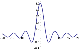
The characteristic function of a uniform U(–1,1) random variable. This function is real-valued because it corresponds to a random variable that is symmetric around the origin; however characteristic functions may generally be complex-valued.

In probability theory and statistics, the characteristic function of any real-valued random variable completely defines its probability distribution. If a random variable admits a probability density function, then the characteristic function is the Fourier transform of the probability density function. Thus it provides an alternative route to analytical results compared with working directly with probability density functions or cumulative distribution functions. There are particularly simple results for the characteristic functions of distributions defined by the weighted sums of random variables.

In addition to univariate distributions, characteristic functions can be defined for vector- or matrix-valued random variables, and can also be extended to more generic cases.

The characteristic function always exists when treated as a function of a real-valued argument, unlike the moment-generating function. There are relations between the behavior of the characteristic function of a distribution and properties of the distribution, such as the existence of moments and the existence of a density function.

Introduction[edit]

The characteristic function is a way for describing a random variable.
The characteristic function,

$varphi _{X}(t)=operatorname {E} left[e^{itX}right],$

a function of t,
completely determines the behavior and properties of the probability distribution of the random variable X.
The characteristic function is similar to the cumulative distribution function,

$F_{X}(x)=operatorname {E} left[mathbf {1} _{{Xleq x}}right]$

(where 1_{{X ≤ x}} is the indicator function — it is equal to 1 when X ≤ x, and zero otherwise), which also completely determines the behavior and properties of the probability distribution of the random variable X. The two approaches are equivalent in the sense that knowing one of the functions it is always possible to find the other, yet they provide different insights for understanding the features of the random variable. Moreover, in particular cases, there can be differences in whether these functions can be represented as expressions involving simple standard functions.

If a random variable admits a density function, then the characteristic function is its Fourier dual, in the sense that each of them is a Fourier transform of the other. If a random variable has a moment-generating function $M_{X}(t)$ , then the domain of the characteristic function can be extended to the complex plane, and

$varphi _{X}(-it)=M_{X}(t).$ ^[1]

Note however that the characteristic function of a distribution always exists, even when the probability density function or moment-generating function do not.

The characteristic function approach is particularly useful in analysis of linear combinations of independent random variables: a classical proof of the Central Limit Theorem uses characteristic functions and Lévy’s continuity theorem. Another important application is to the theory of the decomposability of random variables.

Definition[edit]

For a scalar random variable X the characteristic function is defined as the expected value of e^itX, where i is the imaginary unit, and t ∈ R is the argument of the characteristic function:

${displaystyle {begin{cases}displaystyle varphi _{X}!:mathbb {R} to mathbb {C} \displaystyle varphi _{X}(t)=operatorname {E} left[e^{itX}right]=int _{mathbb {R} }e^{itx},dF_{X}(x)=int _{mathbb {R} }e^{itx}f_{X}(x),dx=int _{0}^{1}e^{itQ_{X}(p)},dpend{cases}}}$

Here F_X is the cumulative distribution function of X, f_X is the corresponding probability density function, Q_X(p) is the corresponding inverse cumulative distribution function also called the quantile function,^[2] and the integrals are of the Riemann–Stieltjes kind. If a random variable X has a probability density function then the characteristic function is its Fourier transform with sign reversal in the complex exponential^[3]^{[page needed]}.^[4] This convention for the constants appearing in the definition of the characteristic function differs from the usual convention for the Fourier transform.^[5] For example, some authors^[6] define φ_X(t) = Ee^−2πitX, which is essentially a change of parameter. Other notation may be encountered in the literature: as the characteristic function for a probability measure p, or as the characteristic function corresponding to a density f.

Characteristic functions were first systematically studied by Paul Lévy, although they were used by others before him. It provides an extremely powerful tool in probability in general, and in asymptotic theory in particular. The power of the characteristic function derives from a set of highly convenient properties. Like the mgf, it determines a distribution. But unlike mgfs, existence is not an issue, and it is a bounded function. It is easily transportable for common functions of random variables, such as convolutions. And it can be used to prove convergence of distributions, as well as to recognize the name of a limiting distribution.

Generalizations[edit]

The notion of characteristic functions generalizes to multivariate random variables and more complicated random elements. The argument of the characteristic function will always belong to the continuous dual of the space where the random variable X takes its values. For common cases such definitions are listed below:

Examples[edit]

Distribution	Characteristic function φ(t)
Degenerate δ_a	${displaystyle e^{ita}}$
Bernoulli Bern(p)	${displaystyle 1-p+pe^{it}}$
Binomial B(n, p)	${displaystyle (1-p+pe^{it})^{n}}$
Negative binomial NB(r, p)	${displaystyle left({frac {p}{1-e^{it}+pe^{it}}}right)^{r}}$
Poisson Pois(λ)	${displaystyle e^{lambda (e^{it}-1)}}$
Uniform (continuous) U(a, b)	${displaystyle {frac {e^{itb}-e^{ita}}{it(b-a)}}}$
Uniform (discrete) DU(a, b)	${displaystyle {frac {e^{ita}-e^{it(b+1)}}{(1-e^{it})(b-a+1)}}}$
Laplace L(μ, b)	${displaystyle {frac {e^{itmu }}{1+b^{2}t^{2}}}}$
Logistic Logistic(μ,s)	${displaystyle e^{imu t}{frac {pi st}{sinh(pi st)}}}$
Normal N(μ, σ²)	${displaystyle e^{itmu -{frac {1}{2}}sigma ^{2}t^{2}}}$
Chi-squared χ²_k	${displaystyle (1-2it)^{-k/2}}$
Noncentral Chi-squared χ^‘2_k	${displaystyle e^{frac {ilambda t}{1-2it}}(1-2it)^{-k/2}}$
Cauchy C(μ, θ)	${displaystyle e^{itmu -theta \|t\|}}$
Gamma Γ(k, θ)	${displaystyle (1-ittheta )^{-k}}$
Exponential Exp(λ)	${displaystyle (1-itlambda ^{-1})^{-1}}$
Geometric Gf(p) (number of failures)	${displaystyle {frac {p}{1-e^{it}(1-p)}}}$
Geometric Gt(p) (number of trials)	${displaystyle {frac {p}{e^{-it}-(1-p)}}}$
Multivariate normal N(μ, Σ)	${displaystyle e^{i{mathbf {t} ^{mathrm {T} }{boldsymbol {mu }}}-{frac {1}{2}}mathbf {t} ^{mathrm {T} }{boldsymbol {Sigma }}mathbf {t} }}$
Multivariate Cauchy MultiCauchy(μ, Σ)^[10]	${displaystyle e^{imathbf {t} ^{mathrm {T} }{boldsymbol {mu }}-{sqrt {mathbf {t} ^{mathrm {T} }{boldsymbol {Sigma }}mathbf {t} }}}}$

Oberhettinger (1973) provides extensive tables of characteristic functions.

Properties[edit]

The characteristic function of a real-valued random variable always exists, since it is an integral of a bounded continuous function over a space whose measure is finite.
A characteristic function is uniformly continuous on the entire space.
It is non-vanishing in a region around zero: φ(0) = 1.
It is bounded: |φ(t)| ≤ 1.
It is Hermitian: φ(−t) = φ(t). In particular, the characteristic function of a symmetric (around the origin) random variable is real-valued and even.
There is a bijection between probability distributions and characteristic functions. That is, for any two random variables X₁, X₂, both have the same probability distribution if and only if $varphi _{X_{1}}=varphi _{X_{2}}$ .
If a random variable X has moments up to k-th order, then the characteristic function φ_X is k times continuously differentiable on the entire real line. In this case

${displaystyle operatorname {E} [X^{k}]=i^{-k}varphi _{X}^{(k)}(0).}$
If a characteristic function φ_X has a k-th derivative at zero, then the random variable X has all moments up to k if k is even, but only up to k – 1 if k is odd.^[11]

${displaystyle varphi _{X}^{(k)}(0)=i^{k}operatorname {E} [X^{k}]}$
If X₁, …, X_n are independent random variables, and a₁, …, a_n are some constants, then the characteristic function of the linear combination of the X_i ‘s is

${displaystyle varphi _{a_{1}X_{1}+cdots +a_{n}X_{n}}(t)=varphi _{X_{1}}(a_{1}t)cdots varphi _{X_{n}}(a_{n}t).}$

One specific case is the sum of two independent random variables X₁ and X₂ in which case one has

${displaystyle varphi _{X_{1}+X_{2}}(t)=varphi _{X_{1}}(t)cdot varphi _{X_{2}}(t).}$
Let and be two random variables with characteristic functions ${displaystyle varphi _{X}}$ and ${displaystyle varphi _{Y}}$ . and are independent if and only if ${displaystyle varphi _{X,Y}(s,t)=varphi _{X}(s)varphi _{Y}(t)quad {text{ for all }}quad (s,t)in mathbb {R} ^{2}}$ .
The tail behavior of the characteristic function determines the smoothness of the corresponding density function.
Let the random variable be the linear transformation of a random variable . The characteristic function of is ${displaystyle varphi _{Y}(t)=e^{itb}varphi _{X}(at)}$ . For random vectors and (where A is a constant matrix and B a constant vector), we have ${displaystyle varphi _{Y}(t)=e^{it^{top }B}varphi _{X}(A^{top }t)}$ .^[12]

Continuity[edit]

The bijection stated above between probability distributions and characteristic functions is sequentially continuous. That is, whenever a sequence of distribution functions F_j(x) converges (weakly) to some distribution F(x), the corresponding sequence of characteristic functions φ_j(t) will also converge, and the limit φ(t) will correspond to the characteristic function of law F. More formally, this is stated as

Lévy’s continuity theorem: A sequence X_j of n-variate random variables converges in distribution to random variable X if and only if the sequence φ_{X_j} converges pointwise to a function φ which is continuous at the origin. Where φ is the characteristic function of X.^[13]

This theorem can be used to prove the law of large numbers and the central limit theorem.

Inversion formula[edit]

There is a one-to-one correspondence between cumulative distribution functions and characteristic functions, so it is possible to find one of these functions if we know the other. The formula in the definition of characteristic function allows us to compute φ when we know the distribution function F (or density f). If, on the other hand, we know the characteristic function φ and want to find the corresponding distribution function, then one of the following inversion theorems can be used.

Theorem. If the characteristic function φ_X of a random variable X is integrable, then F_X is absolutely continuous, and therefore X has a probability density function. In the univariate case (i.e. when X is scalar-valued) the density function is given by

${displaystyle f_{X}(x)=F_{X}'(x)={frac {1}{2pi }}int _{mathbf {R} }e^{-itx}varphi _{X}(t),dt.}$

In the multivariate case it is

${displaystyle f_{X}(x)={frac {1}{(2pi )^{n}}}int _{mathbf {R} ^{n}}e^{-i(tcdot x)}varphi _{X}(t)lambda (dt)}$

where is the dot product.

The density function is the Radon–Nikodym derivative of the distribution μ_X with respect to the Lebesgue measure λ:

${displaystyle f_{X}(x)={frac {dmu _{X}}{dlambda }}(x).}$

Theorem (Lévy).^{[note 1]} If φ_X is characteristic function of distribution function F_X, two points a < b are such that {x | a < x < b} is a continuity set of μ_X (in the univariate case this condition is equivalent to continuity of F_X at points a and b), then

Theorem. If a is (possibly) an atom of X (in the univariate case this means a point of discontinuity of F_X ) then

If X is scalar:

${displaystyle F_{X}(a)-F_{X}(a-0)=lim _{Tto infty }{frac {1}{2T}}int _{-T}^{+T}e^{-ita}varphi _{X}(t),dt}$
If X is a vector random variable:^[15]

${displaystyle mu _{X}({a})=lim _{T_{1}to infty }cdots lim _{T_{n}to infty }left(prod _{k=1}^{n}{frac {1}{2T_{k}}}right)int limits _{[-T_{1},T_{1}]times dots times [-T_{n},T_{n}]}e^{-i(tcdot a)}varphi _{X}(t)lambda (dt)}$

Theorem (Gil-Pelaez).^[16] For a univariate random variable X, if x is a continuity point of F_X then

${displaystyle F_{X}(x)={frac {1}{2}}-{frac {1}{pi }}int _{0}^{infty }{frac {operatorname {Im} [e^{-itx}varphi _{X}(t)]}{t}},dt}$

where the imaginary part of a complex number is given by $mathrm {Im} (z)=(z-z^{*})/2i$ .

And its density function is:

${displaystyle f_{X}(x)={frac {1}{pi }}int _{0}^{infty }operatorname {Re} [e^{-itx}varphi _{X}(t)],dt}$

The integral may be not Lebesgue-integrable; for example, when X is the discrete random variable that is always 0, it becomes the Dirichlet integral.

Inversion formulas for multivariate distributions are available.^[14]^[17]

Criteria for characteristic functions[edit]

The set of all characteristic functions is closed under certain operations:

It is well known that any non-decreasing càdlàg function F with limits F(−∞) = 0, F(+∞) = 1 corresponds to a cumulative distribution function of some random variable. There is also interest in finding similar simple criteria for when a given function φ could be the characteristic function of some random variable. The central result here is Bochner’s theorem, although its usefulness is limited because the main condition of the theorem, non-negative definiteness, is very hard to verify. Other theorems also exist, such as Khinchine’s, Mathias’s, or Cramér’s, although their application is just as difficult. Pólya’s theorem, on the other hand, provides a very simple convexity condition which is sufficient but not necessary. Characteristic functions which satisfy this condition are called Pólya-type.^[18]

Bochner’s theorem. An arbitrary function φ : Rⁿ → C is the characteristic function of some random variable if and only if φ is positive definite, continuous at the origin, and if φ(0) = 1.

Khinchine’s criterion. A complex-valued, absolutely continuous function φ, with φ(0) = 1, is a characteristic function if and only if it admits the representation

${displaystyle varphi (t)=int _{mathbf {R} }g(t+theta ){overline {g(theta )}},dtheta .}$

Mathias’ theorem. A real-valued, even, continuous, absolutely integrable function φ, with φ(0) = 1, is a characteristic function if and only if

${displaystyle (-1)^{n}left(int _{mathbf {R} }varphi (pt)e^{-t^{2}/2}H_{2n}(t),dtright)geq 0}$

for n = 0,1,2,…, and all p > 0. Here H_2n denotes the Hermite polynomial of degree 2n.

Pólya’s theorem can be used to construct an example of two random variables whose characteristic functions coincide over a finite interval but are different elsewhere.

Pólya’s theorem. If varphi is a real-valued, even, continuous function which satisfies the conditions

then φ(t) is the characteristic function of an absolutely continuous distribution symmetric about 0.

Uses[edit]

Because of the continuity theorem, characteristic functions are used in the most frequently seen proof of the central limit theorem. The main technique involved in making calculations with a characteristic function is recognizing the function as the characteristic function of a particular distribution.

Basic manipulations of distributions[edit]

Characteristic functions are particularly useful for dealing with linear functions of independent random variables. For example, if X₁, X₂, …, X_n is a sequence of independent (and not necessarily identically distributed) random variables, and

$S_{n}=sum _{i=1}^{n}a_{i}X_{i},,!$

where the a_i are constants, then the characteristic function for S_n is given by

$varphi _{S_{n}}(t)=varphi _{X_{1}}(a_{1}t)varphi _{X_{2}}(a_{2}t)cdots varphi _{X_{n}}(a_{n}t),!$

In particular, φ_X+Y(t) = φ_X(t)φ_Y(t). To see this, write out the definition of characteristic function:

${displaystyle varphi _{X+Y}(t)=operatorname {E} left[e^{it(X+Y)}right]=operatorname {E} left[e^{itX}e^{itY}right]=operatorname {E} left[e^{itX}right]operatorname {E} left[e^{itY}right]=varphi _{X}(t)varphi _{Y}(t)}$

The independence of X and Y is required to establish the equality of the third and fourth expressions.

Another special case of interest for identically distributed random variables is when a_i = 1/n and then S_n is the sample mean. In this case, writing X for the mean,

$varphi _{overline {X}}(t)=varphi _{X}!left({tfrac {t}{n}}right)^{n}$

Moments[edit]

Characteristic functions can also be used to find moments of a random variable. Provided that the n^th moment exists, the characteristic function can be differentiated n times and

${displaystyle left[{frac {d^{n}}{dt^{n}}}varphi _{X}(t)right]_{t=0}=i^{n}operatorname {E} left[X^{n}right]Rightarrow operatorname {E} left[X^{n}right]=i^{-n}left[{frac {d^{n}}{dt^{n}}}varphi _{X}(t)right]_{t=0}=i^{-n}varphi _{X}^{(n)}(0),!}$

For example, suppose X has a standard Cauchy distribution. Then φ_X(t) = e^−|t|. This is not differentiable at t = 0, showing that the Cauchy distribution has no expectation. Also, the characteristic function of the sample mean X of n independent observations has characteristic function φ_X(t) = (e^−|t|/n)ⁿ = e^−|t|, using the result from the previous section. This is the characteristic function of the standard Cauchy distribution: thus, the sample mean has the same distribution as the population itself.

As a further example, suppose X follows a Gaussian distribution i.e. ${displaystyle Xsim {mathcal {N}}(mu ,sigma ^{2})}$ . Then ${displaystyle varphi _{X}(t)=e^{mu it-{frac {1}{2}}sigma ^{2}t^{2}}}$ and

${displaystyle operatorname {E} left[Xright]=i^{-1}left[{frac {d}{dt}}varphi _{X}(t)right]_{t=0}=i^{-1}left[(imu -sigma ^{2}t)varphi _{X}(t)right]_{t=0}=mu }$

A similar calculation shows ${displaystyle operatorname {E} left[X^{2}right]=mu ^{2}+sigma ^{2}}$ and is easier to carry out than applying the definition of expectation and using integration by parts to evaluate ${displaystyle operatorname {E} left[X^{2}right]}$ .

The logarithm of a characteristic function is a cumulant generating function, which is useful for finding cumulants; some instead define the cumulant generating function as the logarithm of the moment-generating function, and call the logarithm of the characteristic function the second cumulant generating function.

Data analysis[edit]

Characteristic functions can be used as part of procedures for fitting probability distributions to samples of data. Cases where this provides a practicable option compared to other possibilities include fitting the stable distribution since closed form expressions for the density are not available which makes implementation of maximum likelihood estimation difficult. Estimation procedures are available which match the theoretical characteristic function to the empirical characteristic function, calculated from the data. Paulson et al. (1975)^[19] and Heathcote (1977)^[20] provide some theoretical background for such an estimation procedure. In addition, Yu (2004)^[21] describes applications of empirical characteristic functions to fit time series models where likelihood procedures are impractical. Empirical characteristic functions have also been used by Ansari et al. (2020)^[22] and Li et al. (2020)^[23] for training generative adversarial networks.

Example[edit]

The gamma distribution with scale parameter θ and a shape parameter k has the characteristic function

${displaystyle (1-theta it)^{-k}.}$

Now suppose that we have

${displaystyle X~sim Gamma (k_{1},theta ){mbox{ and }}Ysim Gamma (k_{2},theta )}$

with X and Y independent from each other, and we wish to know what the distribution of X + Y is. The characteristic functions are

${displaystyle varphi _{X}(t)=(1-theta it)^{-k_{1}},,qquad varphi _{Y}(t)=(1-theta it)^{-k_{2}}}$

which by independence and the basic properties of characteristic function leads to

${displaystyle varphi _{X+Y}(t)=varphi _{X}(t)varphi _{Y}(t)=(1-theta it)^{-k_{1}}(1-theta it)^{-k_{2}}=left(1-theta itright)^{-(k_{1}+k_{2})}.}$

This is the characteristic function of the gamma distribution scale parameter θ and shape parameter k₁ + k₂, and we therefore conclude

${displaystyle X+Ysim Gamma (k_{1}+k_{2},theta )}$

The result can be expanded to n independent gamma distributed random variables with the same scale parameter and we get

$forall iin {1,ldots ,n}:X_{i}sim Gamma (k_{i},theta )qquad Rightarrow qquad sum _{i=1}^{n}X_{i}sim Gamma left(sum _{i=1}^{n}k_{i},theta right).$

Entire characteristic functions[edit]

This section needs expansion. You can help by adding to it. (December 2009)

As defined above, the argument of the characteristic function is treated as a real number: however, certain aspects of the theory of characteristic functions are advanced by extending the definition into the complex plane by analytical continuation, in cases where this is possible.^[24]

[edit]

Related concepts include the moment-generating function and the probability-generating function. The characteristic function exists for all probability distributions. This is not the case for the moment-generating function.

The characteristic function is closely related to the Fourier transform: the characteristic function of a probability density function p(x) is the complex conjugate of the continuous Fourier transform of p(x) (according to the usual convention; see continuous Fourier transform – other conventions).

$varphi _{X}(t)=langle e^{itX}rangle =int _{mathbf {R} }e^{itx}p(x),dx={overline {left(int _{mathbf {R} }e^{-itx}p(x),dxright)}}={overline {P(t)}},$

where P(t) denotes the continuous Fourier transform of the probability density function p(x). Likewise, p(x) may be recovered from φ_X(t) through the inverse Fourier transform:

$p(x)={frac {1}{2pi }}int _{mathbf {R} }e^{itx}P(t),dt={frac {1}{2pi }}int _{mathbf {R} }e^{itx}{overline {varphi _{X}(t)}},dt.$

Indeed, even when the random variable does not have a density, the characteristic function may be seen as the Fourier transform of the measure corresponding to the random variable.

Another related concept is the representation of probability distributions as elements of a reproducing kernel Hilbert space via the kernel embedding of distributions. This framework may be viewed as a generalization of the characteristic function under specific choices of the kernel function.

Notes[edit]

^ named after the French mathematician Paul Lévy

References[edit]

Citations[edit]

^ Lukacs (1970), p. 196.
^ Shaw, W. T.; McCabe, J. (2009). «Monte Carlo sampling given a Characteristic Function: Quantile Mechanics in Momentum Space». arXiv:0903.1592 [q-fin.CP].
^ Statistical and Adaptive Signal Processing (2005)
^ Billingsley (1995).
^ Pinsky (2002).
^ Bochner (1955).
^ Andersen et al. (1995), Definition 1.10.
^ Andersen et al. (1995), Definition 1.20.
^ Sobczyk (2001), p. 20.
^ Kotz & Nadarajah (2004), p. 37 using 1 as the number of degree of freedom to recover the Cauchy distribution
^ Lukacs (1970), Corollary 1 to Theorem 2.3.1.
^ «Joint characteristic function». www.statlect.com. Retrieved 7 April 2018.
^ Cuppens (1975), Theorem 2.6.9.
^ ^a ^b ^c Shephard (1991a).
^ Cuppens (1975), Theorem 2.3.2.
^ Wendel (1961).
^ Shephard (1991b).
^ Lukacs (1970), p. 84.
^ Paulson, Holcomb & Leitch (1975).
^ Heathcote (1977).
^ Yu (2004).
^ Ansari, Scarlett & Soh (2020).
^ Li et al. (2020).
^ Lukacs (1970), Chapter 7.

Sources[edit]

Andersen, H.H.; Højbjerre, M.; Sørensen, D.; Eriksen, P.S. (1995). Linear and graphical models for the multivariate complex normal distribution. Lecture Notes in Statistics 101. New York: Springer-Verlag. ISBN 978-0-387-94521-7.
Billingsley, Patrick (1995). Probability and measure (3rd ed.). John Wiley & Sons. ISBN 978-0-471-00710-4.
Bisgaard, T. M.; Sasvári, Z. (2000). Characteristic functions and moment sequences. Nova Science.
Bochner, Salomon (1955). Harmonic analysis and the theory of probability. University of California Press.
Cuppens, R. (1975). Decomposition of multivariate probabilities. Academic Press. ISBN 9780121994501.
Heathcote, C.R. (1977). «The integrated squared error estimation of parameters». Biometrika. 64 (2): 255–264. doi:10.1093/biomet/64.2.255.
Lukacs, E. (1970). Characteristic functions. London: Griffin.
Kotz, Samuel; Nadarajah, Saralees (2004). Multivariate T Distributions and Their Applications. Cambridge University Press.
Manolakis, Dimitris G.; Ingle, Vinay K.; Kogon, Stephen M. (2005). Statistical and Adaptive Signal Processing: Spectral Estimation, Signal Modeling, Adaptive Filtering, and Array Processing. Artech House. ISBN 978-1-58053-610-3.
Oberhettinger, Fritz (1973). Fourier transforms of distributions and their inverses; a collection of tables. New York: Academic Press. ISBN 9780125236508.
Paulson, A.S.; Holcomb, E.W.; Leitch, R.A. (1975). «The estimation of the parameters of the stable laws». Biometrika. 62 (1): 163–170. doi:10.1093/biomet/62.1.163.
Pinsky, Mark (2002). Introduction to Fourier analysis and wavelets. Brooks/Cole. ISBN 978-0-534-37660-4.
Sobczyk, Kazimierz (2001). Stochastic differential equations. Kluwer Academic Publishers. ISBN 978-1-4020-0345-5.
Wendel, J.G. (1961). «The non-absolute convergence of Gil-Pelaez’ inversion integral». The Annals of Mathematical Statistics. 32 (1): 338–339. doi:10.1214/aoms/1177705164.
Yu, J. (2004). «Empirical characteristic function estimation and its applications». Econometrics Reviews. 23 (2): 93–1223. doi:10.1081/ETC-120039605. S2CID 9076760.
Shephard, N. G. (1991a). «From characteristic function to distribution function: A simple framework for the theory». Econometric Theory. 7 (4): 519–529. doi:10.1017/s0266466600004746. S2CID 14668369.
Shephard, N. G. (1991b). «Numerical integration rules for multivariate inversions». J. Statist. Comput. Simul. 39 (1–2): 37–46. doi:10.1080/00949659108811337.
Ansari, Abdul Fatir; Scarlett, Jonathan; Soh, Harold (2020). «A Characteristic Function Approach to Deep Implicit Generative Modeling». Proceedings of the IEEE/CVF Conference on Computer Vision and Pattern Recognition (CVPR), 2020. pp. 7478–7487.
Li, Shengxi; Yu, Zeyang; Xiang, Min; Mandic, Danilo (2020). «Reciprocal Adversarial Learning via Characteristic Functions». Advances in Neural Information Processing Systems 33 (NeurIPS 2020).

External links[edit]

«Characteristic function», Encyclopedia of Mathematics, EMS Press, 2001 [1994]

Источник

Характеристическая функция случайной величины

Примеры решений: характеристическая функция

3.1. Характеристическая функция биномиального закона.

3.2. Характеристическая функция закона Пуассона.

3.3. Характеристическая функция геометрического закона.

Introduction[edit]

Definition[edit]

Generalizations[edit]

Examples[edit]

Properties[edit]

Continuity[edit]

Inversion formula[edit]

Criteria for characteristic functions[edit]

Uses[edit]

Basic manipulations of distributions[edit]

Moments[edit]

Data analysis[edit]

Example[edit]

Entire characteristic functions[edit]

[edit]

See also[edit]

Notes[edit]

References[edit]

Citations[edit]

Sources[edit]

External links[edit]

Не пропустите также: