Как найти электропроводность вещества - Avtoru.top

Почему медь проводит электричество лучше, чем вода? Прочитав эту статью, вы больше не будете задавать себе больше этот вопрос. Далее мы обсудим электропроводность и рассмотрим формулы, которые описывают это понятие. Наконец, вы можете проверить свои знания на двух примерах.

Простое объяснение.

Электропроводность — это физическая величина, которая описывает насколько хорошо определенный материал проводит электричество.

Формулы

Существует три различных формульных обозначения удельной электропроводности σ (греч. сигма), k (каппа) и γ (гамма). В дальнейшем мы будем использовать σ. Формула электропроводности, также называемой удельной электропроводностью, описывается формулой:

σ = 1 / ρ .

Здесь ρ называется удельным сопротивлением. Вы можете рассчитать электрическое сопротивление R проводника с учетом его параметров следующим образом: R = ( ρ * l ) / S .

Таким образом, сопротивление R равно удельному сопротивлению ρ , умноженному на длину проводника l, деленному на площадь поперечного сечения S. Если теперь вы хотите выразить эту формулу через удельную электропроводность σ = 1 / ρ , полезно знать, что электрическая проводимость G проводника выражается следующим образом: G = 1 / R .

Если в верхнюю формулу подставить удельную электропроводность σ и электрическую проводимость G, то получится следующее: 1 / G = ( 1 / σ ) * ( l / S ) .

Путем дальнейшего преобразования можно получить выражение: G = σ * S / l .

С помощью электропроводности можно также описать важную зависимость между плотностью электрического тока и напряженностью электрического поля с помощью выражения: J = σ * E .

Единица измерения

Единицей удельной электропроводности σ в СИ является: [ σ ] = 1 См/м ( Сименс на метр ).

Эти единицы определяются по формуле G = σ * S / l . Если решить эту формулу в соответствии с σ, то получим σ = G * l / S .

Единица измерения электрической проводимости G задается как: [ G ] = 1 / σ = 1 См ( Сименс, международное обозначение: S ).

Если теперь ввести в формулу все единицы измерения, то получится:

[ σ ] = 1 См * 1 м / м² = 1 См / м .

Вы также будете чаще использовать единицы измерения См / см , м / Ом * мм² или См * м / мм² . Вы можете преобразовать отдельные измеряемые переменные так: См / см = См / 10^-2 м и так: м / Ом * мм² = См * м / мм² = См * м / 10^-3 м * 10^-3 м = 10⁶ См / м .

Электропроводность металлов

В зависимости от количества свободно перемещающихся электронов один материал проводит лучше, чем другой. В принципе, любой материал является проводящим, но в изоляторах, например, протекающий электрический ток ничтожно мал, поэтому здесь мы говорим о непроводниках.

В металлических связях валентные электроны, т.е. крайние электроны в атоме, свободно подвижны. Они расположены в так называемой полосе проводимости. Находящиеся там электроны образуют так называемый электронный газ. Соответственно, металлы являются сравнительно хорошими проводниками. Если теперь подать электрическое напряжение на металл, валентные электроны медленно движутся к положительному полюсу, потому что он их притягивает.

Рис. 1. Движение электронов в металле

На рисунке 1 видно, что некоторые электроны не могут быть притянуты непосредственно к положительному полюсу, потому что на пути стоит, так сказать, твердое атомное ядро. Там они замедляются и в некоторой степени отклоняются. Именно поэтому электроны не могут ускоряться в металле бесконечно, и именно так возникает удельное сопротивление или электропроводность.

Теперь вы также можете измерить удельную электропроводность в металле с помощью следующей формулы: σ = ( n * e² * τ ) / m .

В этой формуле n означает число электронов, e — заряд электрона, m — массу электрона, а τ — среднее время полета электрона между двумя столкновениями.

Таблица удельной электропроводности

Для большинства веществ уже известны значения удельной электропроводности. Некоторые из них вы можете найти в следующей таблице ниже. Все значения в этой таблице действительны для комнатной температуры, т.е. 25°C.

Вещество	Удельная электропроводность в См / м
Серебро	62 · 10⁶
Медь	58 · 10⁶
Золото	45,2 · 10⁶
Алюминий	37,7 · 10⁶
Вольфрам	19 · 10⁶
Латунь	15,5 · 10⁶
Железо	9,93 · 10⁶
Нержавеющая сталь (WNr. 1,4301)	1,36 · 10⁶
Германий (легирование <10^-9)	2
Кремний (легирование <10^-12)	0,5 · 10^-3
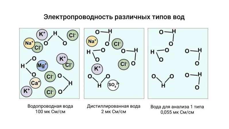
Морская вода	примерно 5
Водопроводная вода	примерно 0,05
Дистиллированная вода	5 · 10^-6
Изолятор	обычно <10^-8

Таблица удельной электропроводности некоторых веществ при температуре 25 °C

Удельная электропроводность сильно зависит от температуры, поэтому указанные значения применимы только при 25°C. При повышении температуры вибрация решетки в веществе становится выше. Это нарушает поток электронов, и поэтому электропроводность уменьшается с ростом температуры.

Из таблицы видно, что медь имеет вторую по величине электропроводность, поэтому медные кабели очень часто используются в электротехнике. Серебро обладает еще более высокой проводимостью, но стоит намного дороже меди.

Интересно также сравнение между морской и дистиллированной водой. Здесь электропроводность возникает благодаря растворенным в воде ионам. Морская вода имеет очень высокую долю соли, которая растворяется в воде. Эти ионы передают электрический ток. В дистиллированной воде нет растворенных ионов, поэтому в ней практически не может протекать электрический ток. Поэтому электропроводность морской воды намного выше, чем дистиллированной.

Примеры задач

Для более детального рассмотрения приведём два примера расчетов.

Задача 1.

В первой задаче представьте, что у вас есть провод длиной 2 м с поперечным сечением 0,5 мм². Электрическое сопротивление провода при комнатной температуре составляет 106 мОм. Из какого материала изготовлен провод?

Решение.

Решение данной задачи можно найти с помощью формулы: R = ( 1 / σ ) * ( l / S ). Из этой формулы найдём σ = l / ( S * R ) .

Теперь вы можете вставить заданные значения, убедившись, что вы перевели сечение в м².

σ = l / ( S * R ) = 2 м / ( ( 0,5 * 10^-6 м² ) * ( 1 / 106 * 10^-3 Ом ) ) = 37, 7 * 10⁶ См / м .

Наконец, вы ищите в таблице, какой материал имеет удельную электропроводность σ = 37, 7 * 10⁶ См / м и приходите к выводу, что провод сделан из алюминия.

Задача 2.

В задаче 2 вам дано только удельное сопротивление образца с 735 * 10^-9 Ом * м. Из какого материла изготовлен образец?

Решение.

Вы можете использовать формулу σ = 1 / ρ для расчёта удельной электропроводности. После подстановки значений в эту формулу вы получите: σ = 1 / ρ = 1 / 735 * 10^-9 Ом * м = 1,36 * 10⁶ См / м .

Если вы снова заглянете в таблицу, то обнаружите, что образец должен быть изготовлен из нержавеющей стали.

Источник

Электропроводность растворов, что такое и как измерить?

Что такое электропроводность?

Электропроводность – это способность вещества проводить электрический ток. В аналитической химии чаще всего говорят об электропроводности растворов, то есть его способности проводить электрический ток. Относительная дешевизна, надежность и быстрый отклик приборов для измерения электропроводности сделали их популярным аналитическим инструментом, который есть практически в каждой лаборатории.

Чистые растворители практически не проводят электрический ток, и их электрическая проводимость стремится к нулю. Заряд в растворе переносят ионы или вещества с сильнополярными связями. При растворении твердых полярных веществ в воде происходит электролитическая диссоциация, то есть распад молекул на катионы и анионы. По степени распада на ионы различают сильные и слабые электролиты. Сильные электролиты диссоциируют полностью с образованием ионов. Слабые электролиты диссоциируют частично с образованием ионов и сохранением не ионной молекулы. Способностью проводить ток обладают только ионы, недиссоциированные молекулы не участвуют в электрической проводимости. Вклад иона в проводимость раствора можно описать функцией от его концентрации, заряда и подвижности иона.

k = f(c * z * λ)

Как измеряется электропроводность растворов?

Электропроводность — это величина обратно пропорциональная сопротивлению. Согласно закону Ома, сопротивление рассчитывается как отношение силы тока к напряжению. Таким образом, измерив силу тока и зная напряжение, можно рассчитать электропроводность. Для её измерения используют специальные приборы — кондуктометры. Кондуктометры измеряют силу тока, проходящую между электродами через раствор при известном напряжении. Различные производители, исследователи и инженеры разрабатывают и используют электроды различной геометрической формы и конфигурации. Чтобы полученные на разных приборах значения можно было сравнивать между собой, прибор автоматически преобразует измеренную фактическую электропроводность в удельную электропроводность. Удельная электропроводность раствора – это электропроводность слоя раствора длинной 1 см между электродами площадью 1 см².

Чувствительный элемент кондуктометра — кондуктометрический датчик представляет с собой два электрода (иногда четыре), на которые подаёте напряжение, а измерительный прибор (кондуктометр) измеряет силу тока и рассчитывает удельную электропроводность.

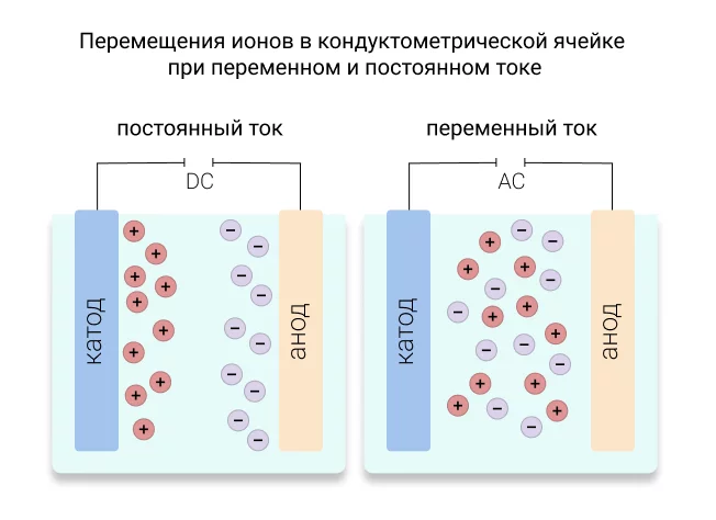
Если на электроды подать постоянный ток, то на положительно заряженном электроде (аноде) будут накапливаться анионы, а на отрицательно заряженном электроде (катоде) будут накапливаться катионы. Такое накопление ионов у электрода приведет к их электролизу и изменению состава анализируемой жидкости, как следствие изменится и электропроводность. Для предотвращения нежелательных реакций на поверхностях электродов, на них подается переменный ток. Под действием переменного тока ионы не движутся в одном направлении, они колеблются в такт частоты приложенного тока. Современные кондуктометры настраивают частоту переменного тока автоматически.

Каждый кондуктометрический датчик имеет свой калибровочный коэффициент, который зависит от формы электродов, расстояния между ними и их состояния. Этот коэффициент также называют константой кондуктометрической ячейки. При производстве новой кондуктометрической ячейки ей присваивается расчётная (номинальная) константа кондуктометрической ячейки. Перед первым измерением необходимо выполнить калибровку кондуктометра, кондуктометр запишет действительную константу ячейки в память и автоматически будет использовать её при дальнейшем расчете удельной электропроводности.

Полный текст статьи «Измерение электропроводности растворов, калибровка кондуктометра» читайте на labex.su

Источник

This article is about electrical conductivity in general. For other types of conductivity, see Conductivity. For specific applications in electrical elements, see Electrical resistance and conductance.

Resistivity
Common symbols	ρ
SI unit	ohm metre (Ω⋅m)
In SI base units	kg⋅m³⋅s⁻³⋅A⁻²
Derivations from other quantities	${displaystyle rho =R{frac {A}{ell }}}$
Dimension	${displaystyle {mathsf {M}}{mathsf {L}}^{3}{mathsf {T}}^{-3}{mathsf {I}}^{-2}}$

Conductivity
Common symbols	σ, κ, γ
SI unit	siemens per metre (S/m)
In SI base units	kg⁻¹⋅m⁻³⋅s³⋅A²
Derivations from other quantities	${displaystyle sigma ={frac {1}{rho }}}$
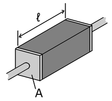
Dimension	${displaystyle {mathsf {M}}^{-1}{mathsf {L}}^{-3}{mathsf {T}}^{3}{mathsf {I}}^{2}}$

Electrical resistivity (also called specific electrical resistance or volume resistivity) is a fundamental property of a material that measures how strongly it resists electric current. A low resistivity indicates a material that readily allows electric current. Resistivity is commonly represented by the Greek letter ρ (rho). The SI unit of electrical resistivity is the ohm-meter (Ω⋅m).^[1]^[2]^[3] For example, if a 1 m³ solid cube of material has sheet contacts on two opposite faces, and the resistance between these contacts is 1 Ω, then the resistivity of the material is 1 Ω⋅m.

Electrical conductivity (or specific conductance) is the reciprocal of electrical resistivity. It represents a material’s ability to conduct electric current. It is commonly signified by the Greek letter σ (sigma), but κ (kappa) (especially in electrical engineering) and γ (gamma) are sometimes used. The SI unit of electrical conductivity is siemens per metre (S/m). Resistivity and conductivity are intensive properties of materials, giving the opposition of a standard cube of material to current. Electrical resistance and conductance are corresponding extensive properties that give the opposition of a specific object to electric current.

Definition[edit]

Ideal case[edit]

A piece of resistive material with electrical contacts on both ends.

In an ideal case, cross-section and physical composition of the examined material are uniform across the sample, and the electric field and current density are both parallel and constant everywhere. Many resistors and conductors do in fact have a uniform cross section with a uniform flow of electric current, and are made of a single material, so that this is a good model. (See the adjacent diagram.) When this is the case, the electrical resistivity ρ (Greek: rho) can be calculated by:

${displaystyle rho =R{frac {A}{ell }},}$

where

The resistivity can be expressed using the SI unit ohm metre (Ω⋅m) — i.e. ohms multiplied by square metres (for the cross-sectional area) then divided by metres (for the length).

Both resistance and resistivity describe how difficult it is to make electrical current flow through a material, but unlike resistance, resistivity is an intrinsic property. This means that all pure copper wires (which have not been subjected to distortion of their crystalline structure etc.), irrespective of their shape and size, have the same resistivity, but a long, thin copper wire has a much larger resistance than a thick, short copper wire. Every material has its own characteristic resistivity. For example, rubber has a far larger resistivity than copper.

In a hydraulic analogy, passing current through a high-resistivity material is like pushing water through a pipe full of sand — while passing current through a low-resistivity material is like pushing water through an empty pipe. If the pipes are the same size and shape, the pipe full of sand has higher resistance to flow. Resistance, however, is not solely determined by the presence or absence of sand. It also depends on the length and width of the pipe: short or wide pipes have lower resistance than narrow or long pipes.

The above equation can be transposed to get Pouillet’s law (named after Claude Pouillet):

${displaystyle R=rho {frac {ell }{A}}.}$

The resistance of a given element is proportional to the length, but inversely proportional to the cross-sectional area. For example, if A = 1 m², ell = 1 m (forming a cube with perfectly conductive contacts on opposite faces), then the resistance of this element in ohms is numerically equal to the resistivity of the material it is made of in Ω⋅m.

Conductivity, σ, is the inverse of resistivity:

${displaystyle sigma ={frac {1}{rho }}.}$

Conductivity has SI units of siemens per metre (S/m).

General scalar quantities[edit]

For less ideal cases, such as more complicated geometry, or when the current and electric field vary in different parts of the material, it is necessary to use a more general expression in which the resistivity at a particular point is defined as the ratio of the electric field to the density of the current it creates at that point:

${displaystyle rho ={frac {E}{J}},}$

where

in which and are inside the conductor.

Conductivity is the inverse (reciprocal) of resistivity. Here, it is given by:

${displaystyle sigma ={frac {1}{rho }}={frac {J}{E}}.}$

For example, rubber is a material with large ρ and small σ — because even a very large electric field in rubber makes almost no current flow through it. On the other hand, copper is a material with small ρ and large σ — because even a small electric field pulls a lot of current through it.

As shown below, this expression simplifies to a single number when the electric field and current density are constant in the material.

Derivation from general definition of resistivity
There are three equations to be combined here. The first is the resistivity for parallel current and electric field: ${displaystyle rho ={frac {E}{J}},}$ If the electric field is constant, the electric field is given by the total voltage V across the conductor divided by length ℓ of the conductor: ${displaystyle E={frac {V}{ell }}.}$ If the current density is constant, it is equal to the total current divided by the cross sectional area: ${displaystyle J={frac {I}{A}}.}$ Plugging in the values of E and J into the first expression, we obtain: ${displaystyle rho ={frac {VA}{Iell }}.}$ Finally, we apply Ohm’s law, V/I = R: ${displaystyle rho =R{frac {A}{ell }}.}$

Derivation from general definition of resistivity

There are three equations to be combined here. The first is the resistivity for parallel current and electric field:

${displaystyle rho ={frac {E}{J}},}$

If the electric field is constant, the electric field is given by the total voltage V across the conductor divided by length ℓ of the conductor:

${displaystyle E={frac {V}{ell }}.}$

If the current density is constant, it is equal to the total current divided by the cross sectional area:

${displaystyle J={frac {I}{A}}.}$

Plugging in the values of E and J into the first expression, we obtain:

${displaystyle rho ={frac {VA}{Iell }}.}$

Finally, we apply Ohm’s law, V/I = R:

${displaystyle rho =R{frac {A}{ell }}.}$

Tensor resistivity[edit]

When the resistivity of a material has a directional component, the most general definition of resistivity must be used. It starts from the tensor-vector form of Ohm’s law, which relates the electric field inside a material to the electric current flow. This equation is completely general, meaning it is valid in all cases, including those mentioned above. However, this definition is the most complicated, so it is only directly used in anisotropic cases, where the more simple definitions cannot be applied. If the material is not anisotropic, it is safe to ignore the tensor-vector definition, and use a simpler expression instead.

Here, anisotropic means that the material has different properties in different directions. For example, a crystal of graphite consists microscopically of a stack of sheets, and current flows very easily through each sheet, but much less easily from one sheet to the adjacent one.^[4] In such cases, the current does not flow in exactly the same direction as the electric field. Thus, the appropriate equations are generalized to the three-dimensional tensor form:^[5]^[6]

where the conductivity σ and resistivity ρ are rank-2 tensors, and electric field E and current density J are vectors. These tensors can be represented by 3×3 matrices, the vectors with 3×1 matrices, with matrix multiplication used on the right side of these equations. In matrix form, the resistivity relation is given by:

${displaystyle {begin{bmatrix}E_{x}\E_{y}\E_{z}end{bmatrix}}={begin{bmatrix}rho _{xx}&rho _{xy}&rho _{xz}\rho _{yx}&rho _{yy}&rho _{yz}\rho _{zx}&rho _{zy}&rho _{zz}end{bmatrix}}{begin{bmatrix}J_{x}\J_{y}\J_{z}end{bmatrix}},}$

where

Equivalently, resistivity can be given in the more compact Einstein notation:

${displaystyle mathbf {E} _{i}={boldsymbol {rho }}_{ij}mathbf {J} _{j}~.}$

In either case, the resulting expression for each electric field component is:

${displaystyle {begin{aligned}E_{x}&=rho _{xx}J_{x}+rho _{xy}J_{y}+rho _{xz}J_{z}\E_{y}&=rho _{yx}J_{x}+rho _{yy}J_{y}+rho _{yz}J_{z}\E_{z}&=rho _{zx}J_{x}+rho _{zy}J_{y}+rho _{zz}J_{z}end{aligned}}.}$

Since the choice of the coordinate system is free, the usual convention is to simplify the expression by choosing an x-axis parallel to the current direction, so J_y = J_z = 0. This leaves:

${displaystyle rho _{xx}={frac {E_{x}}{J_{x}}},quad rho _{yx}={frac {E_{y}}{J_{x}}},{text{ and }}rho _{zx}={frac {E_{z}}{J_{x}}}.}$

Conductivity is defined similarly:^[7]

${displaystyle {begin{bmatrix}J_{x}\J_{y}\J_{z}end{bmatrix}}={begin{bmatrix}sigma _{xx}&sigma _{xy}&sigma _{xz}\sigma _{yx}&sigma _{yy}&sigma _{yz}\sigma _{zx}&sigma _{zy}&sigma _{zz}end{bmatrix}}{begin{bmatrix}E_{x}\E_{y}\E_{z}end{bmatrix}}}$

${displaystyle mathbf {J} _{i}={boldsymbol {sigma }}_{ij}mathbf {E} _{j},}$

both resulting in:

${displaystyle {begin{aligned}J_{x}&=sigma _{xx}E_{x}+sigma _{xy}E_{y}+sigma _{xz}E_{z}\J_{y}&=sigma _{yx}E_{x}+sigma _{yy}E_{y}+sigma _{yz}E_{z}\J_{z}&=sigma _{zx}E_{x}+sigma _{zy}E_{y}+sigma _{zz}E_{z}end{aligned}}.}$

Looking at the two expressions, and are the matrix inverse of each other. However, in the most general case, the individual matrix elements are not necessarily reciprocals of one another; for example, σ_xx may not be equal to 1/ρ_xx. This can be seen in the Hall effect, where ${displaystyle rho _{xy}}$ is nonzero. In the Hall effect, due to rotational invariance about the z-axis, ${displaystyle rho _{yy}=rho _{xx}}$ and ${displaystyle rho _{yx}=-rho _{xy}}$ , so the relation between resistivity and conductivity simplifies to:^[8]

${displaystyle sigma _{xx}={frac {rho _{xx}}{rho _{xx}^{2}+rho _{xy}^{2}}},quad sigma _{xy}={frac {-rho _{xy}}{rho _{xx}^{2}+rho _{xy}^{2}}}.}$

If the electric field is parallel to the applied current, ${displaystyle rho _{xy}}$ and ${displaystyle rho _{xz}}$ are zero. When they are zero, one number, ${displaystyle rho _{xx}}$ , is enough to describe the electrical resistivity. It is then written as simply rho , and this reduces to the simpler expression.

Conductivity and current carriers[edit]

Relation between current density and electric current velocity[edit]

Electric current is the ordered movement of electric charges.^[2]

Causes of conductivity[edit]

Band theory simplified[edit]

According to elementary quantum mechanics, an electron in an atom or crystal can only have certain precise energy levels; energies between these levels are impossible. When a large number of such allowed levels have close-spaced energy values – i.e. have energies that differ only minutely – those close energy levels in combination are called an «energy band». There can be many such energy bands in a material, depending on the atomic number of the constituent atoms^[a] and their distribution within the crystal.^[b]

The material’s electrons seek to minimize the total energy in the material by settling into low energy states; however, the Pauli exclusion principle means that only one can exist in each such state. So the electrons «fill up» the band structure starting from the bottom. The characteristic energy level up to which the electrons have filled is called the Fermi level. The position of the Fermi level with respect to the band structure is very important for electrical conduction: Only electrons in energy levels near or above the Fermi level are free to move within the broader material structure, since the electrons can easily jump among the partially occupied states in that region. In contrast, the low energy states are completely filled with a fixed limit on the number of electrons at all times, and the high energy states are empty of electrons at all times.

Electric current consists of a flow of electrons. In metals there are many electron energy levels near the Fermi level, so there are many electrons available to move. This is what causes the high electronic conductivity of metals.

An important part of band theory is that there may be forbidden bands of energy: energy intervals that contain no energy levels. In insulators and semiconductors, the number of electrons is just the right amount to fill a certain integer number of low energy bands, exactly to the boundary. In this case, the Fermi level falls within a band gap. Since there are no available states near the Fermi level, and the electrons are not freely movable, the electronic conductivity is very low.

In metals[edit]

Like balls in a Newton’s cradle, electrons in a metal quickly transfer energy from one terminal to another, despite their own negligible movement.

A metal consists of a lattice of atoms, each with an outer shell of electrons that freely dissociate from their parent atoms and travel through the lattice. This is also known as a positive ionic lattice.^[9] This ‘sea’ of dissociable electrons allows the metal to conduct electric current. When an electrical potential difference (a voltage) is applied across the metal, the resulting electric field causes electrons to drift towards the positive terminal. The actual drift velocity of electrons is typically small, on the order of magnitude of metres per hour. However, due to the sheer number of moving electrons, even a slow drift velocity results in a large current density.^[10] The mechanism is similar to transfer of momentum of balls in a Newton’s cradle^[11] but the rapid propagation of an electric energy along a wire is not due to the mechanical forces, but the propagation of an energy-carrying electromagnetic field guided by the wire.

Most metals have electrical resistance. In simpler models (non quantum mechanical models) this can be explained by replacing electrons and the crystal lattice by a wave-like structure. When the electron wave travels through the lattice, the waves interfere, which causes resistance. The more regular the lattice is, the less disturbance happens and thus the less resistance. The amount of resistance is thus mainly caused by two factors. First, it is caused by the temperature and thus amount of vibration of the crystal lattice. Higher temperatures cause bigger vibrations, which act as irregularities in the lattice. Second, the purity of the metal is relevant as a mixture of different ions is also an irregularity.^[12]^[13] The small decrease in conductivity on melting of pure metals is due to the loss of long range crystalline order. The short range order remains and strong correlation between positions of ions results in coherence between waves diffracted by adjacent ions.^[14]

In semiconductors and insulators[edit]

In metals, the Fermi level lies in the conduction band (see Band Theory, above) giving rise to free conduction electrons. However, in semiconductors the position of the Fermi level is within the band gap, about halfway between the conduction band minimum (the bottom of the first band of unfilled electron energy levels) and the valence band maximum (the top of the band below the conduction band, of filled electron energy levels). That applies for intrinsic (undoped) semiconductors. This means that at absolute zero temperature, there would be no free conduction electrons, and the resistance is infinite. However, the resistance decreases as the charge carrier density (i.e., without introducing further complications, the density of electrons) in the conduction band increases. In extrinsic (doped) semiconductors, dopant atoms increase the majority charge carrier concentration by donating electrons to the conduction band or producing holes in the valence band. (A «hole» is a position where an electron is missing; such holes can behave in a similar way to electrons.) For both types of donor or acceptor atoms, increasing dopant density reduces resistance. Hence, highly doped semiconductors behave metallically. At very high temperatures, the contribution of thermally generated carriers dominates over the contribution from dopant atoms, and the resistance decreases exponentially with temperature.

In ionic liquids/electrolytes[edit]

In electrolytes, electrical conduction happens not by band electrons or holes, but by full atomic species (ions) traveling, each carrying an electrical charge. The resistivity of ionic solutions (electrolytes) varies tremendously with concentration – while distilled water is almost an insulator, salt water is a reasonable electrical conductor. Conduction in ionic liquids is also controlled by the movement of ions, but here we are talking about molten salts rather than solvated ions. In biological membranes, currents are carried by ionic salts. Small holes in cell membranes, called ion channels, are selective to specific ions and determine the membrane resistance.

The concentration of ions in a liquid (e.g., in an aqueous solution) depends on the degree of dissociation of the dissolved substance, characterized by a dissociation coefficient alpha , which is the ratio of the concentration of ions to the concentration of molecules of the dissolved substance $N_{0}$ :

${displaystyle N=alpha N_{0}~.}$

The specific electrical conductivity ( sigma ) of a solution is equal to:

${displaystyle sigma =qleft(b^{+}+b^{-}right)alpha N_{0}~,}$

where : module of the ion charge, ${displaystyle b^{+}}$ and ${displaystyle b^{-}}$ : mobility of positively and negatively charged ions, $N_{0}$ : concentration of molecules of the dissolved substance, alpha : the coefficient of dissociation.

Superconductivity[edit]

Original data from the 1911 experiment by Heike Kamerlingh Onnes showing the resistance of a mercury wire as a function of temperature. The abrupt drop in resistance is the superconducting transition.

The electrical resistivity of a metallic conductor decreases gradually as temperature is lowered. In normal (that is, non-superconducting) conductors, such as copper or silver, this decrease is limited by impurities and other defects. Even near absolute zero, a real sample of a normal conductor shows some resistance. In a superconductor, the resistance drops abruptly to zero when the material is cooled below its critical temperature. In a normal conductor, the current is driven by a voltage gradient, whereas in a superconductor, there is no voltage gradient and the current is instead related to the phase gradient of the superconducting order parameter.^[15] A consequence of this is that an electric current flowing in a loop of superconducting wire can persist indefinitely with no power source.^[16]

In a class of superconductors known as type II superconductors, including all known high-temperature superconductors, an extremely low but nonzero resistivity appears at temperatures not too far below the nominal superconducting transition when an electric current is applied in conjunction with a strong magnetic field, which may be caused by the electric current. This is due to the motion of magnetic vortices in the electronic superfluid, which dissipates some of the energy carried by the current. The resistance due to this effect is tiny compared with that of non-superconducting materials, but must be taken into account in sensitive experiments. However, as the temperature decreases far enough below the nominal superconducting transition, these vortices can become frozen so that the resistance of the material becomes truly zero.

Plasma[edit]

Lightning is an example of plasma present at Earth’s surface. Typically, lightning discharges 30,000 amperes at up to 100 million volts, and emits light, radio waves, and X-rays.^[17] Plasma temperatures in lightning might approach 30,000 kelvin (29,727 °C) (53,540 °F), or five times hotter than the temperature at the sun surface, and electron densities may exceed 10²⁴ m⁻³.

Plasmas are very good conductors and electric potentials play an important role.

The potential as it exists on average in the space between charged particles, independent of the question of how it can be measured, is called the plasma potential, or space potential. If an electrode is inserted into a plasma, its potential generally lies considerably below the plasma potential, due to what is termed a Debye sheath. The good electrical conductivity of plasmas makes their electric fields very small. This results in the important concept of quasineutrality, which says the density of negative charges is approximately equal to the density of positive charges over large volumes of the plasma (n_e = ⟨Z⟩>n_i), but on the scale of the Debye length there can be charge imbalance. In the special case that double layers are formed, the charge separation can extend some tens of Debye lengths.

The magnitude of the potentials and electric fields must be determined by means other than simply finding the net charge density. A common example is to assume that the electrons satisfy the Boltzmann relation:

${displaystyle n_{text{e}}propto exp left(ePhi /k_{text{B}}T_{text{e}}right).}$

Differentiating this relation provides a means to calculate the electric field from the density:

${displaystyle mathbf {E} =-{frac {k_{text{B}}T_{text{e}}}{e}}{frac {nabla n_{text{e}}}{n_{text{e}}}}.}$

(∇ is the vector gradient operator; see nabla symbol and gradient for more information.)

It is possible to produce a plasma that is not quasineutral. An electron beam, for example, has only negative charges. The density of a non-neutral plasma must generally be very low, or it must be very small. Otherwise, the repulsive electrostatic force dissipates it.

In astrophysical plasmas, Debye screening prevents electric fields from directly affecting the plasma over large distances, i.e., greater than the Debye length. However, the existence of charged particles causes the plasma to generate, and be affected by, magnetic fields. This can and does cause extremely complex behavior, such as the generation of plasma double layers, an object that separates charge over a few tens of Debye lengths. The dynamics of plasmas interacting with external and self-generated magnetic fields are studied in the academic discipline of magnetohydrodynamics.

Plasma is often called the fourth state of matter after solid, liquids and gases.^[18]^[19] It is distinct from these and other lower-energy states of matter. Although it is closely related to the gas phase in that it also has no definite form or volume, it differs in a number of ways, including the following:

Property	Gas	Plasma
Electrical conductivity	Very low: air is an excellent insulator until it breaks down into plasma at electric field strengths above 30 kilovolts per centimetre.^[20]	Usually very high: for many purposes, the conductivity of a plasma may be treated as infinite.
Independently acting species	One: all gas particles behave in a similar way, influenced by gravity and by collisions with one another.	Two or three: electrons, ions, protons and neutrons can be distinguished by the sign and value of their charge so that they behave independently in many circumstances, with different bulk velocities and temperatures, allowing phenomena such as new types of waves and instabilities.
Velocity distribution	Maxwellian: collisions usually lead to a Maxwellian velocity distribution of all gas particles, with very few relatively fast particles.	Often non-Maxwellian: collisional interactions are often weak in hot plasmas and external forcing can drive the plasma far from local equilibrium and lead to a significant population of unusually fast particles.
Interactions	Binary: two-particle collisions are the rule, three-body collisions extremely rare.	Collective: waves, or organized motion of plasma, are very important because the particles can interact at long ranges through the electric and magnetic forces.

Resistivity and conductivity of various materials[edit]

A conductor such as a metal has high conductivity and a low resistivity.
An insulator like glass has low conductivity and a high resistivity.
The conductivity of a semiconductor is generally intermediate, but varies widely under different conditions, such as exposure of the material to electric fields or specific frequencies of light, and, most important, with temperature and composition of the semiconductor material.

The degree of semiconductors doping makes a large difference in conductivity. To a point, more doping leads to higher conductivity. The conductivity of a water/aqueous solution is highly dependent on its concentration of dissolved salts, and other chemical species that ionize in the solution. Electrical conductivity of water samples is used as an indicator of how salt-free, ion-free, or impurity-free the sample is; the purer the water, the lower the conductivity (the higher the resistivity). Conductivity measurements in water are often reported as specific conductance, relative to the conductivity of pure water at 25 °C. An EC meter is normally used to measure conductivity in a solution. A rough summary is as follows:

This table shows the resistivity (ρ), conductivity and temperature coefficient of various materials at 20 °C (68 °F; 293 K).

The effective temperature coefficient varies with temperature and purity level of the material. The 20 °C value is only an approximation when used at other temperatures. For example, the coefficient becomes lower at higher temperatures for copper, and the value 0.00427 is commonly specified at 0 °C.^[52]

The extremely low resistivity (high conductivity) of silver is characteristic of metals. George Gamow tidily summed up the nature of the metals’ dealings with electrons in his popular science book One, Two, Three…Infinity (1947):

The metallic substances differ from all other materials by the fact that the outer shells of their atoms are bound rather loosely, and often let one of their electrons go free. Thus the interior of a metal is filled up with a large number of unattached electrons that travel aimlessly around like a crowd of displaced persons. When a metal wire is subjected to electric force applied on its opposite ends, these free electrons rush in the direction of the force, thus forming what we call an electric current.

More technically, the free electron model gives a basic description of electron flow in metals.

Wood is widely regarded as an extremely good insulator, but its resistivity is sensitively dependent on moisture content, with damp wood being a factor of at least 10¹⁰ worse insulator than oven-dry.^[45] In any case, a sufficiently high voltage – such as that in lightning strikes or some high-tension power lines – can lead to insulation breakdown and electrocution risk even with apparently dry wood.^{[citation needed]}

Temperature dependence[edit]

Linear approximation[edit]

The electrical resistivity of most materials changes with temperature. If the temperature T does not vary too much, a linear approximation is typically used:

${displaystyle rho (T)=rho _{0}[1+alpha (T-T_{0})],}$

where alpha is called the temperature coefficient of resistivity, $T_{0}$ is a fixed reference temperature (usually room temperature), and $rho _{0}$ is the resistivity at temperature $T_{0}$ . The parameter alpha is an empirical parameter fitted from measurement data, equal to 1/ kappa ^[clarify]. Because the linear approximation is only an approximation, alpha is different for different reference temperatures. For this reason it is usual to specify the temperature that alpha was measured at with a suffix, such as $alpha _{15}$ , and the relationship only holds in a range of temperatures around the reference.^[53] When the temperature varies over a large temperature range, the linear approximation is inadequate and a more detailed analysis and understanding should be used.

Metals[edit]

In general, electrical resistivity of metals increases with temperature. Electron–phonon interactions can play a key role. At high temperatures, the resistance of a metal increases linearly with temperature. As the temperature of a metal is reduced, the temperature dependence of resistivity follows a power law function of temperature. Mathematically the temperature dependence of the resistivity ρ of a metal can be approximated through the Bloch–Grüneisen formula:^[54]

${displaystyle rho (T)=rho (0)+Aleft({frac {T}{Theta _{R}}}right)^{n}int _{0}^{Theta _{R}/T}{frac {x^{n}}{(e^{x}-1)(1-e^{-x})}},dx,}$

where rho (0) is the residual resistivity due to defect scattering, A is a constant that depends on the velocity of electrons at the Fermi surface, the Debye radius and the number density of electrons in the metal. $Theta _{R}$ is the Debye temperature as obtained from resistivity measurements and matches very closely with the values of Debye temperature obtained from specific heat measurements. n is an integer that depends upon the nature of interaction:

n = 5 implies that the resistance is due to scattering of electrons by phonons (as it is for simple metals)
n = 3 implies that the resistance is due to s-d electron scattering (as is the case for transition metals)
n = 2 implies that the resistance is due to electron–electron interaction.

The Bloch–Grüneisen formula is an approximation obtained assuming that the studied metal has spherical Fermi surface inscribed within the first Brillouin zone and a Debye phonon spectrum.^[55]

If more than one source of scattering is simultaneously present, Matthiessen’s rule (first formulated by Augustus Matthiessen in the 1860s)^[56]^[57] states that the total resistance can be approximated by adding up several different terms, each with the appropriate value of n.

As the temperature of the metal is sufficiently reduced (so as to ‘freeze’ all the phonons), the resistivity usually reaches a constant value, known as the residual resistivity. This value depends not only on the type of metal, but on its purity and thermal history. The value of the residual resistivity of a metal is decided by its impurity concentration. Some materials lose all electrical resistivity at sufficiently low temperatures, due to an effect known as superconductivity.

An investigation of the low-temperature resistivity of metals was the motivation to Heike Kamerlingh Onnes’s experiments that led in 1911 to discovery of superconductivity. For details see History of superconductivity.

Wiedemann–Franz law[edit]

The Wiedemann–Franz law states that for materials where heat and charge transport is dominated by electrons, the ratio of thermal to electrical conductivity is proportional to the temperature:

${displaystyle {kappa over sigma }={pi ^{2} over 3}left({frac {k}{e}}right)^{2}T,}$

where kappa is the thermal conductivity, is the Boltzmann constant, is the electron charge, is temperature, and sigma is the electric conductivity. The ratio on the rhs is called the Lorenz number.

Semiconductors[edit]

In general, intrinsic semiconductor resistivity decreases with increasing temperature. The electrons are bumped to the conduction energy band by thermal energy, where they flow freely, and in doing so leave behind holes in the valence band, which also flow freely. The electric resistance of a typical intrinsic (non doped) semiconductor decreases exponentially with temperature:

${displaystyle rho =rho _{0}e^{-aT}.}$

An even better approximation of the temperature dependence of the resistivity of a semiconductor is given by the Steinhart–Hart equation:

${displaystyle {frac {1}{T}}=A+Bln rho +C(ln rho )^{3},}$

where A, B and C are the so-called Steinhart–Hart coefficients.

This equation is used to calibrate thermistors.

Extrinsic (doped) semiconductors have a far more complicated temperature profile. As temperature increases starting from absolute zero they first decrease steeply in resistance as the carriers leave the donors or acceptors. After most of the donors or acceptors have lost their carriers, the resistance starts to increase again slightly due to the reducing mobility of carriers (much as in a metal). At higher temperatures, they behave like intrinsic semiconductors as the carriers from the donors/acceptors become insignificant compared to the thermally generated carriers.^[58]

In non-crystalline semiconductors, conduction can occur by charges quantum tunnelling from one localised site to another. This is known as variable range hopping and has the characteristic form of

${displaystyle rho =Aexp left(T^{-{frac {1}{n}}}right),}$

where n = 2, 3, 4, depending on the dimensionality of the system.

Complex resistivity and conductivity[edit]

When analyzing the response of materials to alternating electric fields (dielectric spectroscopy),^[59] in applications such as electrical impedance tomography,^[60] it is convenient to replace resistivity with a complex quantity called impedivity (in analogy to electrical impedance). Impedivity is the sum of a real component, the resistivity, and an imaginary component, the reactivity (in analogy to reactance). The magnitude of impedivity is the square root of sum of squares of magnitudes of resistivity and reactivity.

Conversely, in such cases the conductivity must be expressed as a complex number (or even as a matrix of complex numbers, in the case of anisotropic materials) called the admittivity. Admittivity is the sum of a real component called the conductivity and an imaginary component called the susceptivity.

An alternative description of the response to alternating currents uses a real (but frequency-dependent) conductivity, along with a real permittivity. The larger the conductivity is, the more quickly the alternating-current signal is absorbed by the material (i.e., the more opaque the material is). For details, see Mathematical descriptions of opacity.

Resistance versus resistivity in complicated geometries[edit]

Even if the material’s resistivity is known, calculating the resistance of something made from it may, in some cases, be much more complicated than the formula above. One example is spreading resistance profiling, where the material is inhomogeneous (different resistivity in different places), and the exact paths of current flow are not obvious.

In cases like this, the formulas

must be replaced with

where E and J are now vector fields. This equation, along with the continuity equation for J and the Poisson’s equation for E, form a set of partial differential equations. In special cases, an exact or approximate solution to these equations can be worked out by hand, but for very accurate answers in complex cases, computer methods like finite element analysis may be required.

Resistivity-density product[edit]

In some applications where the weight of an item is very important, the product of resistivity and density is more important than absolute low resistivity – it is often possible to make the conductor thicker to make up for a higher resistivity; and then a low-resistivity-density-product material (or equivalently a high conductivity-to-density ratio) is desirable. For example, for long-distance overhead power lines, aluminium is frequently used rather than copper (Cu) because it is lighter for the same conductance.

Silver, although it is the least resistive metal known, has a high density and performs similarly to copper by this measure, but is much more expensive. Calcium and the alkali metals have the best resistivity-density products, but are rarely used for conductors due to their high reactivity with water and oxygen (and lack of physical strength). Aluminium is far more stable. Toxicity excludes the choice of beryllium.^[61] (Pure beryllium is also brittle.) Thus, aluminium is usually the metal of choice when the weight or cost of a conductor is the driving consideration.

Notes[edit]

^ The atomic number is the count of electrons in an atom that is electrically neutral – has no net electric charge.
^ Other relevant factors that are specifically not considered are the size of the whole crystal and external factors of the surrounding environment that modify the energy bands, such as imposed electric or magnetic fields.
^ The numbers in this column increase or decrease the significand portion of the resistivity. For example, at 30 °C (303 K), the resistivity of silver is 1.65×10⁻⁸. This is calculated as Δρ = α ΔT ρ₀ where ρ₀ is the resistivity at 20 °C (in this case) and α is the temperature coefficient.
^ The conductivity of metallic silver is not significantly better than metallic copper for most practical purposes – the difference between the two can be easily compensated for by thickening the copper wire by only 3%. However silver is preferred for exposed electrical contact points because corroded silver is a tolerable conductor, but corroded copper is a fairly good insulator, like most corroded metals.
^ Copper is widely used in electrical equipment, building wiring, and telecommunication cables.
^ Referred to as 100% IACS or International Annealed Copper Standard. The unit for expressing the conductivity of nonmagnetic materials by testing using the eddy current method. Generally used for temper and alloy verification of aluminium.
^ Despite being less conductive than copper, gold is commonly used in electrical contacts because it does not easily corrode.
^ Commonly used for overhead power line with steel reinforced (ACSR)
^ ^a ^b Cobalt and ruthenium are considered to replace copper in integrated circuits fabricated in advanced nodes^[29]
^ 18% chromium and 8% nickel austenitic stainless steel
^ Nickel-iron-chromium alloy commonly used in heating elements.
^ Graphite is strongly anisotropic.
^ ^a ^b The resistivity of semiconductors depends strongly on the presence of impurities in the material.
^ Corresponds to an average salinity of 35 g/kg at 20 °C.
^ The pH should be around 8.4 and the conductivity in the range of 2.5–3 mS/cm. The lower value is appropriate for freshly prepared water. The conductivity is used for the determination of TDS (total dissolved particles).
^ This value range is typical of high quality drinking water and not an indicator of water quality
^ Conductivity is lowest with monatomic gases present; changes to 12×10⁻⁵ upon complete de-gassing, or to 7.5×10⁻⁵ upon equilibration to the atmosphere due to dissolved CO₂

References[edit]

^ Lowrie, William (2007). Fundamentals of Geophysics. Cambridge University Press. pp. 254–55. ISBN 978-05-2185-902-8. Retrieved March 24, 2019.
^ ^a ^b Kumar, Narinder (2003). Comprehensive Physics for Class XII. New Delhi: Laxmi Publications. pp. 280–84. ISBN 978-81-7008-592-8. Retrieved March 24, 2019.
^ Bogatin, Eric (2004). Signal Integrity: Simplified. Prentice Hall Professional. p. 114. ISBN 978-0-13-066946-9. Retrieved March 24, 2019.
^ ^a ^b ^c Hugh O. Pierson, Handbook of carbon, graphite, diamond, and fullerenes: properties, processing, and applications, p. 61, William Andrew, 1993 ISBN 0-8155-1339-9.
^ J.R. Tyldesley (1975) An introduction to Tensor Analysis: For Engineers and Applied Scientists, Longman, ISBN 0-582-44355-5
^ G. Woan (2010) The Cambridge Handbook of Physics Formulas, Cambridge University Press, ISBN 978-0-521-57507-2
^ Josef Pek, Tomas Verner (3 Apr 2007). «Finite‐difference modelling of magnetotelluric fields in two‐dimensional anisotropic media». Geophysical Journal International. 128 (3): 505–521. doi:10.1111/j.1365-246X.1997.tb05314.x.
^ David Tong (Jan 2016). «The Quantum Hall Effect: TIFR Infosys Lectures» (PDF). Retrieved 14 Sep 2018.
^ Bonding (sl). ibchem.com
^ «Current versus Drift Speed». The physics classroom. Retrieved 20 August 2014.
^ Lowe, Doug (2012). Electronics All-in-One For Dummies. John Wiley & Sons. ISBN 978-0-470-14704-7.
^ Keith Welch. «Questions & Answers – How do you explain electrical resistance?». Thomas Jefferson National Accelerator Facility. Retrieved 28 April 2017.
^ «Electromigration : What is electromigration?». Middle East Technical University. Retrieved 31 July 2017. When electrons are conducted through a metal, they interact with imperfections in the lattice and scatter. […] Thermal energy produces scattering by causing atoms to vibrate. This is the source of resistance of metals.
^ Faber, T.E. (1972). Introduction to the Theory of Liquid Metals. Cambridge University Press. ISBN 9780521154499.
^
«The Feynman Lectures in Physics, Vol. III, Chapter 21: The Schrödinger Equation in a Classical Context: A Seminar on Superconductivity». Retrieved 26 December 2021.
^
John C. Gallop (1990). SQUIDS, the Josephson Effects and Superconducting Electronics. CRC Press. pp. 3, 20. ISBN 978-0-7503-0051-3.
^ See Flashes in the Sky: Earth’s Gamma-Ray Bursts Triggered by Lightning
^ Yaffa Eliezer, Shalom Eliezer, The Fourth State of Matter: An Introduction to the Physics of Plasma, Publisher: Adam Hilger, 1989, ISBN 978-0-85274-164-1, 226 pages, page 5
^ Bittencourt, J.A. (2004). Fundamentals of Plasma Physics. Springer. p. 1. ISBN 9780387209753.
^ Hong, Alice (2000). «Dielectric Strength of Air». The Physics Factbook.
^ ^a ^b ^c ^d ^e ^f ^g ^h ⁱ ^j ^k ^l ^m ⁿ ^o Raymond A. Serway (1998). Principles of Physics (2nd ed.). Fort Worth, Texas; London: Saunders College Pub. p. 602. ISBN 978-0-03-020457-9.
^ ^a ^b ^c David Griffiths (1999) [1981]. «7 Electrodynamics». In Alison Reeves (ed.). Introduction to Electrodynamics (3rd ed.). Upper Saddle River, New Jersey: Prentice Hall. p. 286. ISBN 978-0-13-805326-0. OCLC 40251748.
^ Matula, R.A. (1979). «Electrical resistivity of copper, gold, palladium, and silver». Journal of Physical and Chemical Reference Data. 8 (4): 1147. Bibcode:1979JPCRD…8.1147M. doi:10.1063/1.555614. S2CID 95005999.
^ Douglas Giancoli (2009) [1984]. «25 Electric Currents and Resistance». In Jocelyn Phillips (ed.). Physics for Scientists and Engineers with Modern Physics (4th ed.). Upper Saddle River, New Jersey: Prentice Hall. p. 658. ISBN 978-0-13-149508-1.
^ «Copper wire tables». United States National Bureau of Standards. Retrieved 3 February 2014 – via Internet Archive — archive.org (archived 2001-03-10).
^ [1]. (Calculated as «56% conductivity of pure copper» (5.96E-7)). Retrieved on 2023-1-12.
^ Physical constants. (PDF format; see page 2, table in the right lower corner). Retrieved on 2011-12-17.
^ [2]. (Calculated as «28% conductivity of pure copper» (5.96E-7)). Retrieved on 2023-1-12.
^ IITC – Imec Presents Copper, Cobalt and Ruthenium Interconnect Results
^ «Temperature Coefficient of Resistance | Electronics Notes».
^ [3]. (Calculated as «15% conductivity of pure copper» (5.96E-7)). Retrieved on 2023-1-12.
^ Material properties of niobium.
^ AISI 1010 Steel, cold drawn. Matweb
^ Karcher, Ch.; Kocourek, V. (December 2007). «Free-surface instabilities during electromagnetic shaping of liquid metals». Proceedings in Applied Mathematics and Mechanics. 7 (1): 4140009–4140010. doi:10.1002/pamm.200700645. ISSN 1617-7061.
^ «JFE steel» (PDF). Retrieved 2012-10-20.
^ ^a ^b Douglas C. Giancoli (1995). Physics: Principles with Applications (4th ed.). London: Prentice Hall. ISBN 978-0-13-102153-2.
(see also Table of Resistivity. hyperphysics.phy-astr.gsu.edu)
^ John O’Malley (1992) Schaum’s outline of theory and problems of basic circuit analysis, p. 19, McGraw-Hill Professional, ISBN 0-07-047824-4
^ Glenn Elert (ed.), «Resistivity of steel», The Physics Factbook, retrieved and archived 16 June 2011.
^ Probably, the metal with highest value of electrical resistivity.
^ Y. Pauleau, Péter B. Barna, P. B. Barna (1997) Protective coatings and thin films: synthesis, characterization, and applications, p. 215, Springer, ISBN 0-7923-4380-8.
^ Milton Ohring (1995). Engineering materials science, Volume 1 (3rd ed.). Academic Press. p. 561. ISBN 978-0125249959.
^ Physical properties of sea water Archived 2018-01-18 at the Wayback Machine. Kayelaby.npl.co.uk. Retrieved on 2011-12-17.
^ [4]. chemistry.stackexchange.com
^ Eranna, Golla (2014). Crystal Growth and Evaluation of Silicon for VLSI and ULSI. CRC Press. p. 7. ISBN 978-1-4822-3281-3.
^ ^a ^b ^c Transmission Lines data. Transmission-line.net. Retrieved on 2014-02-03.
^ R. M. Pashley; M. Rzechowicz; L. R. Pashley; M. J. Francis (2005). «De-Gassed Water is a Better Cleaning Agent». The Journal of Physical Chemistry B. 109 (3): 1231–8. doi:10.1021/jp045975a. PMID 16851085.
^ ASTM D1125 Standard Test Methods for Electrical Conductivity and Resistivity of Water
^ ASTM D5391 Standard Test Method for Electrical Conductivity and Resistivity of a Flowing High Purity Water Sample
^ Lawrence S. Pan, Don R. Kania, Diamond: electronic properties and applications, p. 140, Springer, 1994 ISBN 0-7923-9524-7.
^ S. D. Pawar; P. Murugavel; D. M. Lal (2009). «Effect of relative humidity and sea level pressure on electrical conductivity of air over Indian Ocean». Journal of Geophysical Research. 114 (D2): D02205. Bibcode:2009JGRD..114.2205P. doi:10.1029/2007JD009716.
^ E. Seran; M. Godefroy; E. Pili (2016). «What we can learn from measurements of air electric conductivity in 222Rn ‐ rich atmosphere». Earth and Space Science. 4 (2): 91–106. Bibcode:2017E&SS….4…91S. doi:10.1002/2016EA000241.
^ Copper Wire Tables Archived 2010-08-21 at the Wayback Machine. US Dep. of Commerce. National Bureau of Standards Handbook. February 21, 1966
^ Ward, Malcolm R. (1971). Electrical engineering science. McGraw-Hill technical education. Maidenhead, UK: McGraw-Hill. pp. 36–40. ISBN 9780070942554.
^ Grüneisen, E. (1933). «Die Abhängigkeit des elektrischen Widerstandes reiner Metalle von der Temperatur». Annalen der Physik. 408 (5): 530–540. Bibcode:1933AnP…408..530G. doi:10.1002/andp.19334080504. ISSN 1521-3889.
^ Quantum theory of real materials. James R. Chelikowsky, Steven G. Louie. Boston: Kluwer Academic Publishers. 1996. pp. 219–250. ISBN 0-7923-9666-9. OCLC 33335083.{{cite book}}: CS1 maint: others (link)
^ A. Matthiessen, Rep. Brit. Ass. 32, 144 (1862)
^ A. Matthiessen, Progg. Anallen, 122, 47 (1864)
^ J. Seymour (1972) Physical Electronics, chapter 2, Pitman
^ Stephenson, C.; Hubler, A. (2015). «Stability and conductivity of self-assembled wires in a transverse electric field». Sci. Rep. 5: 15044. Bibcode:2015NatSR…515044S. doi:10.1038/srep15044. PMC 4604515. PMID 26463476.
^ Otto H. Schmitt, University of Minnesota Mutual Impedivity Spectrometry and the Feasibility of its Incorporation into Tissue-Diagnostic Anatomical Reconstruction and Multivariate Time-Coherent Physiological Measurements. otto-schmitt.org. Retrieved on 2011-12-17.
^ «Berryllium (Be) — Chemical properties, Health and Environmental effects».

External links[edit]

«Electrical Conductivity». Sixty Symbols. Brady Haran for the University of Nottingham. 2010.
Comparison of the electrical conductivity of various elements in WolframAlpha
Partial and total conductivity. «Electrical conductivity» (PDF).

Источник

Лекция 2

Электропроводность (удельная и эквивалентная), ее зависимость от концентрации и температуры. Методы измерения электропроводности.

Подвижность ионов, закон Кольрауша, аномальная подвижность ионов Н₃О⁺ и ОН^—.

Электропроводность К — величина, обратная электрическому сопротивлению R. Так как R = r , то К = × = k

где r — удельное электрическое сопротивление; l — расстояние между электродами; S — площадь электрода; k — удельная электропроводность.

Удельная электропроводность k жидкости — это электропроводность одного кубического сантиметра раствора, заполняющего пространство между плоскими электродами одинаковой, очень большой площади, находящимися на расстоянии 1 см. Кубический сантиметр раствора должен находиться вдали от границ электрода. [k] = Ом^-1× см^-1.

По закону Ома : R = U/I ; U = E× l (Е — напряженность поля, или падение напряжения на 1 см расстояния; l — расстояние между электродами); I = i× S (i — плотность тока, или ток, приходящийся на 1 см² поверхности электрода; S — площадь электрода). Тогда :

k = ; i = k× E

При Е = 1 В/см i = k.

Что такое проводимость?

Чаще всего под проводимостью понимается способность вещества передавать тепло, звук или электричество. В этом материале мы разберём электрическую проводимость (EC), которая представляет собой способность исследуемой среды проводить электрический ток. Небольшие положительно либо отрицательно заряженные частицы, называемые ионами, помогают переносить электрический заряд через вещество. Чем больше таких ионов, тем выше проводимость, соответственно, меньшее количество ионов приводит к снижению проводимости. А чем выше проводимость, тем выше способность среды проводить электричество. Это связано с большим количеством заряженных ионов, присутствующих в образце. Самой высокой электрической проводимостью обладают проводники – металлы и электролиты.

Электропроводность сред, также называемая ЕС, основана на проводимости, которая, как мы выяснили, является способностью вещества передавать ток. Единицами измерения электропроводности является Siemens/cm (S/cm, mS/cm, μS/cm, dS/m). Например, сверхчистая вода имеет удельную проводимость 0.055 μS/см при температуре 25 °С. Величина электропроводности обратна величине электрического сопротивления, несмотря на то, что обе они являются характеристиками электропроводящей способности материалов.

Какие отрасли промышленности полагаются на измерения ЕС?

Теперь давайте взглянем на конкретные применения измерений ЕС в конкретных отраслях жизнедеятельности человека.

Фото: Joe, источник: pixabay.com

ЕС и сельское хозяйство

В сельскохозяйственной промышленности знание электропроводности почвы чрезвычайно важно для здоровья и роста сельскохозяйственных культур. Фермеры и производители, как правило, регулярно производят мониторинг содержания фосфатов, нитратов, кальция и калия почвы, поскольку эти питательные вещества необходимы для успешного роста растений. Тестирование электропроводности (ЕС) почвы может помочь производителям отслеживать количество всех питательных веществ, присутствующих в почве, и определять, требует ли она больше питательных веществ или же, наоборот, имеет место её перенасыщение. Таким образом, измерение EC почвы помогает экономить денежные средства в долгосрочной перспективе и обеспечивает здоровое растениеводство.

EC и обработка воды

Электрическая проводимость играет огромную роль в различных сферах, связанных с контролем качества воды. При очистке сточных вод ЕС измеряется для того, чтобы сопоставить параметры отходящих сточных вод со свойствами воды, в которую они поступают. Попадание в чистую воду стоков с чрезвычайно высокой или низкой солёностью может иметь пагубные последствия для здоровья водной флоры и фауны. Таким образом, сохранение измерений ЕС в приемлемых диапазонах является важным и полезным для поддержания здоровой и устойчивой экосистемы наших океанов и других природных водоёмов.

EC и гальванические ванны

Проводимость может также оказывать воздействие на гальванические ванны, с помощью которых проводятся процедуры нанесения на металлы слоёв защищающих веществ и/или придания им определённой окраски. Поэтому измерения ЕС являются обычным делом в таких отраслях, как аэрокосмическая промышленность, автомобилестроение, изготовление ювелирных изделий и т. д.

Измерения ЕС и общего содержания растворенных твердых веществ (TDS)

Между тем, электропроводимость можно измерять и с целью определения общего количества растворенных твердых веществ в средах (TDS) и их солёности, что также весьма востребовано в различных отраслях промышленности. Обычно измерение EC используется для оценки параметров TDS. Это подразумевает то, что природа твёрдых частиц является ионной и соотношение между растворенными ионами и проводимостью ЕС нам известно.

Для измерения TDS используются единицы мг/л (ppm) или г/л. Некоторые модели измерителей электропроводимости разрешают пользователю осуществлять введение коэффициента TDS для последующего преобразования, однако в большинстве приборов данный коэффициент устанавливается автоматически на значении 0.50. Для растворов с высоким содержанием ионов коэффициент TDS составляет 0.5, а для слабых образцов, таких как, например, удобрения, он равен 0.7. Следует заметить, что коэффициенты преобразования TDS для разных твёрдых тел являются различными.

Фото: Benjamin Thomas, источник: pixabay.com

Измерения электропроводимости и солёности

Измерения EC также могут применяться для определения солёности морской воды. Существуют различные шкалы, предназначенные для измерений солёности в солёной воде в зависимости от возможностей вашего измерительного прибора. Три общих шкалы солености – это практическая шкала минерализации (от 0.00 до 42.00 единиц практической солености, определенных Организацией Объединенных Наций по вопросам образования и культуры (ЮНЕСКО) в 1978 году; процентная шкала (от 0.0 до 400.0 %), где 100 % — морская вода; и природная шкала морской воды (от 0.00 до 80.00 п.п.), определенная ЮНЕСКО в 1966 году. Каждый измеритель электропроводности обладает собственными алгоритмами для преобразования результатов измерений проводимости в желаемый масштаб в соответствии с этими шкалами.

Влияние температуры измеряемого вещества на показатели проводимости

Следует также иметь в виду, что температура измеряемого образца влиять на измерения ЕС. Ведь от температуры зависит активность ионов и концентрация вещества, а это, в свою очередь, влияет на проводимость. Чем выше температура раствора, тем ниже сопротивление (что соответствует более высокой проводимости). И, наоборот, чем ниже температура вещества, тем выше сопротивление (и тем ниже проводимость). Встроенные датчики температуры в приборах для измерения проводимости определяют температуру раствора в режиме реального времени. Встроенная автокомпенсация корректирует измеряемую проводимость до контрольной температуры с помощью фиксированного коэффициента β для линейной компенсации. Более продвинутые измерители проводимости позволяют регулировать β для компенсации различных сред и осуществляют регулировку эталонной температур в максимально широких температурных диапазонах.

Какие датчики используют для измерения проводимости?

Существует несколько типов зондов для измерения проводимости. Они подключаются к корпусу измерительного оборудования для сбора максимально точных показаний.

Амперометрический датчик

Амперометрический датчик – это двухэлектродный зонд, измеряющий проводимость с применением амперометрического метода. Эти два электрода изолированы друг от друга, однако и тот и другой при этом контактируют с раствором, для измерения. Данный зонд функционирует с использованием переменного напряжения на определенной частоте между парой электродов, находящихся в растворе.

Двухэлектродные зонды не требуют большого объёма образца, чтобы полностью покрыть датчики, однако измерительный диапазон таких электродов ограничен. Также если вы тестируете образцы, обладающие переменной электропроводимостью, вам вероятнее всего придётся приобрести более одного двухэлектродного зонда и/или измерительного прибора.

Потенциометрический зонд

Данный измерительный датчик представляет собой четырёхкольцовый зонд, который использует для анализа сред потенциометрический подход. В «кольцо» входят два внешних «приводных» и два внутренних электрода. На внешние электроды подаётся переменный ток для индукции тока через раствор. В свою очередь, внутренняя пара электродов измеряет падение потенциала, вызванное наличием тока. Четырёхдиапазонные зонды могут покрывать более широкий измерительный диапазон (концентрацию ионов) и демонстрируют более высокую степень точности, в сравнении с амперометрическим методом исследования. Однако зонд такого типа потребует большего количества измеряемого вещества.

По материалам Brown, M. (октябрь, 2015). Гальваника: о чём должен знать каждый инженер

Используемые изображения:

1. Фото: firestock

2. Автор: Joe, источник: pixabay.com

3. Автор: Benjamin Thomas, источник: pixabay.com

Источник

Формулы

Единица измерения

Электропроводность металлов

Таблица удельной электропроводности

Примеры задач

Электропроводность растворов, что такое и как измерить?

Что такое электропроводность?

Как измеряется электропроводность растворов?

Definition[edit]

Ideal case[edit]

General scalar quantities[edit]

Tensor resistivity[edit]

Conductivity and current carriers[edit]

Relation between current density and electric current velocity[edit]

Causes of conductivity[edit]

Band theory simplified[edit]

In metals[edit]

In semiconductors and insulators[edit]

In ionic liquids/electrolytes[edit]

Superconductivity[edit]

Plasma[edit]

Resistivity and conductivity of various materials[edit]

Temperature dependence[edit]

Linear approximation[edit]

Metals[edit]

Wiedemann–Franz law[edit]

Semiconductors[edit]

Complex resistivity and conductivity[edit]

Resistance versus resistivity in complicated geometries[edit]

Resistivity-density product[edit]

See also[edit]

Notes[edit]

References[edit]

Further reading[edit]

External links[edit]

Рекомендуемые материалы

Что такое проводимость?

Какие отрасли промышленности полагаются на измерения ЕС?

ЕС и сельское хозяйство

EC и обработка воды

EC и гальванические ванны

Измерения ЕС и общего содержания растворенных твердых веществ (TDS)

Измерения электропроводимости и солёности

Влияние температуры измеряемого вещества на показатели проводимости

Какие датчики используют для измерения проводимости?

Амперометрический датчик

Потенциометрический зонд

Не пропустите также: